Equality of Opportunity in Supervised Learning

Moritz Hardt

Eric Price

Nathan Srebro

October 11, 2016

Abstract

We propose a criterion for discrimination against a specified sensitive attribute in supervised learning, where the goal is to predict some target based on available features. Assuming data about the predictor, target, and membership in the protected group are available, we show how to optimally adjust any learned predictor so as to remove discrimination according to our definition. Our framework also improves incentives by shifting the cost of poor classification from disadvantaged groups to the decision maker, who can respond by improving the classification accuracy. In line with other studies, our notion is oblivious: it depends only on the joint statistics of the predictor, the target and the protected attribute, but not on interpretation of individual features. We study the inherent limits of defining and identifying biases based on such oblivious measures, outlining what can and cannot be inferred from different oblivious tests. We illustrate our notion using a case study of FICO credit scores.

Executive Summary: Machine learning models increasingly influence high-stakes decisions in areas like lending, hiring, and criminal justice, where biases against protected groups—such as race or gender—can perpetuate inequality. Existing approaches, like ignoring protected attributes entirely or enforcing equal acceptance rates across groups, often fail: the first overlooks indirect encodings of bias in other data, while the second sacrifices prediction accuracy, even allowing unfair outcomes where qualified people in one group are rejected to balance numbers. With growing regulatory pressure and public concern, as highlighted in U.S. government reports on big data's risks, there is an urgent need for practical fairness measures that do not undermine the core goal of accurate predictions.

This paper sets out to define and demonstrate new criteria for non-discrimination in supervised learning models, which predict outcomes like loan defaults from features while avoiding bias tied to a protected attribute. It evaluates these criteria through theory, optimization methods, and a real-world case study, showing how to measure bias and adjust models without rebuilding them from scratch.

The authors develop their ideas through theoretical analysis and simulations, grounded in standard supervised learning data—samples of features, protected attributes, and actual outcomes. They focus on binary predictions (yes/no decisions) but extend to scores like credit ratings. Key elements include assuming access to joint statistics of predictions, outcomes, and protected groups (from training or audit data), over a broad scope like historical records spanning years. They avoid delving into feature details or causal assumptions, emphasizing "oblivious" tests based only on observable correlations.

The most important results center on two new fairness notions. First, "equalized odds" requires that prediction error rates—true positives (correctly identifying good outcomes) and false positives (mistakenly identifying bad outcomes)—match across protected groups; this ensures the model performs equally well everywhere without letting group membership sway decisions beyond the true outcome. Second, a milder "equal opportunity" version equalizes only true positive rates for the positive outcome (like approving good loans). Unlike prior methods demanding equal overall acceptance rates, these allow perfect accuracy if available and can be achieved by simple post-processing: adjust thresholds or add randomness to an existing model's outputs based on group membership, minimizing accuracy loss via linear optimization. Theory proves this yields the best possible fair model if starting from an optimal unconstrained one, with quantified bounds on performance drops. A non-identifiability result warns that such correlation-based tests cannot distinguish benign correlations (e.g., wealth predicting defaults independently of race) from proxy discrimination (e.g., using race-linked traits). In a case study of 300,000+ FICO credit scores from 2003, linked to defaults and race (Asian, white, Hispanic, Black), equal opportunity achieved 93% of maximum lender profit at a standard 82% non-default threshold—versus 70% for equal acceptance rates—while boosting approval odds for qualified minorities by 20-30 percentage points versus race-blind thresholds.

These findings mean organizations can deploy fairer models with little hit to performance, unlike rigid parity rules that force inaccurate decisions and may approve unqualified minority applicants while rejecting qualified ones from majority groups. By tying fairness to equal accuracy across groups, the approach reduces risk of legal challenges under anti-discrimination laws, enhances trust in AI-driven decisions, and avoids encoding subtle biases from features like family status. It outperforms expectations from prior work by aligning fairness with business goals, though it may counterintuitively require "corrective" adjustments favoring underrepresented groups to offset uncertainty. In the FICO analysis, raw scores showed majority groups (whites) with 10-20% higher prediction accuracy, confirming real biases that post-processing mitigates without crippling utility.

Leaders should prioritize collecting reliable outcome data and test models against these criteria during audits. For immediate fixes, apply post-processing to existing predictors—it's efficient, privacy-friendly, and preferable to retraining if data improvements stall. Opt for equal opportunity in positive-outcome scenarios like lending, as it balances fairness and profit better than stricter equalized odds (which halves utility here due to accuracy gaps). If options exist, invest first in diverse training data or direct outcome predictors to shrink the fairness-accuracy trade-off; otherwise, pilot post-processed models on subsets. Further analysis of feature causality or expanded datasets could refine decisions.

While the methods are theoretically sound and empirically validated on credit data, limitations include reliance on accurate outcomes (e.g., audited defaults), which may be unavailable or biased in practice. The oblivious focus misses deeper causes, risking false alarms on non-discriminatory correlations, and assumes balanced groups for reliable estimates—small minorities may need more data. Confidence is high for measuring and adjusting observable biases in controlled settings, but readers should pair this with domain experts for causal checks before high-stakes use.

1. Introduction

Section Summary: Machine learning is increasingly used in areas like hiring, lending, and criminal justice, where it can improve predictions but also risks perpetuating or creating biases against protected groups such as those based on race or gender. Common approaches, like ignoring protected attributes or enforcing equal acceptance rates across groups, often fail because they either overlook hidden correlations or sacrifice the accuracy that makes these tools valuable. This paper introduces a new, straightforward way to measure and reduce discrimination in predictive models, one that aligns fairness with accuracy, allows for perfect predictions, and relies only on basic data relationships without needing to inspect the model's inner workings.

As machine learning increasingly affects decisions in domains protected by anti-discrimination law, there is much interest in algorithmically measuring and ensuring fairness in machine learning. In domains such as advertising, credit, employment, education, and criminal justice, machine learning could help obtain more accurate predictions, but its effect on existing biases is not well understood. Although reliance on data and quantitative measures can help quantify and eliminate existing biases, some scholars caution that algorithms can also introduce new biases or perpetuate existing ones [1]. In May 2014, the Obama Administration's Big Data Working Group released a report [2] arguing that discrimination can sometimes "be the inadvertent outcome of the way big data technologies are structured and used" and pointed toward "the potential of encoding discrimination in automated decisions". A subsequent White House report [3] calls for "equal opportunity by design" as a guiding principle in domains such as credit scoring.

Despite the demand, a vetted methodology for avoiding discrimination against protected attributes in machine learning is lacking. A naïve approach might require that the algorithm should ignore all protected attributes such as race, color, religion, gender, disability, or family status. However, this idea of "fairness through unawareness" is ineffective due to the existence of redundant encodings, ways of predicting protected attributes from other features [4].

Another common conception of non-discrimination is demographic parity. Demographic parity requires that a decision—such as accepting or denying a loan application—be independent of the protected attribute. In the case of a binary decision $\widehat{Y}\in{0, 1}$ and a binary protected attribute $A\in{0, 1}, $ this constraint can be formalized by asking that $\Pr{\widehat{Y}=1\mid A=0}=\Pr{\widehat{Y}=1\mid A=1}.$ In other words, membership in a protected class should have no correlation with the decision. Through its various equivalent formalizations this idea appears in numerous papers. Unfortunately, as was already argued by Dwork et al. [5], the notion is seriously flawed on two counts. First, it doesn't ensure fairness. Indeed, the notion permits that we accept qualified applicants in the demographic $A=0$, but unqualified individuals in $A=1, $ so long as the percentages of acceptance match. This behavior can arise naturally, when there is little or no training data available within $A=1.$ Second, demographic parity often cripples the utility that we might hope to achieve. Just imagine the common scenario in which the target variable $Y$ —whether an individual actually defaults or not—is correlated with $A.$ Demographic parity would not allow the ideal predictor $\widehat{Y} = Y, $ which can hardly be considered discriminatory as it represents the actual outcome. As a result, the loss in utility of introducing demographic parity can be substantial.

In this paper, we consider non-discrimination from the perspective of supervised learning, where the goal is to predict a true outcome $Y$ from features $X$ based on labeled training data, while ensuring they are "non-discriminatory" with respect to a specified protected attribute $A$. As in the usual supervised learning setting, we assume that we have access to labeled training data, in our case indicating also the protected attribute $A$. That is, to samples from the joint distribution of $(X, A, Y)$. This data is used to construct a predictor $\widehat{Y}(X)$ or $\widehat{Y}(X, A)$, and we also use such data to test whether it is unfairly discriminatory.

Unlike demographic parity, our notion always allows for the perfectly accurate solution of $\widehat{Y} = Y.$ More broadly, our criterion is easier to achieve the more accurate the predictor $\widehat{Y}$ is, aligning fairness with the central goal in supervised learning of building more accurate predictors.

The notion we propose is "oblivious", in that it is based only on the joint distribution, or joint statistics, of the true target $Y$, the predictions $\widehat{Y}$, and the protected attribute $A$. In particular, it does not evaluate the features in $X$ nor the functional form of the predictor $\widehat{Y}(X)$ nor how it was derived. This matches other tests recently proposed and conducted, including demographic parity and different analyses of common risk scores. In many cases, only oblivious analysis is possible as the functional form of the score and underlying training data are not public. The only information about the score is the score itself, which can then be correlated with the target and protected attribute. Furthermore, even if the features or the functional form are available, going beyond oblivious analysis essentially requires subjective interpretation or casual assumptions about specific features, which we aim to avoid.

1.1 Summary of our contributions

We propose a simple, interpretable, and actionable framework for measuring and removing discrimination based on protected attributes. We argue that, unlike demographic parity, our framework provides a meaningful measure of discrimination, while demonstrating in theory and experiment that we also achieve much higher utility. Our key contributions are as follows:

• We propose an easily checkable and interpretable notion of avoiding discrimination based on protected attributes. Our notion enjoys a natural interpretation in terms of graphical dependency models. It can also be viewed as shifting the burden of uncertainty in classification from the protected class to the decision maker. In doing so, our notion helps to incentivize the collection of better features, that depend more directly on the target rather then the protected attribute, and of data that allows better prediction for all protected classes.
• We give a simple and effective framework for constructing classifiers satisfying our criterion from an arbitrary learned predictor. Rather than changing a possibly complex training pipeline, the result follows via a simple post-processing step that minimizes the loss in utility.
• We show that the Bayes optimal non-discriminating (according to our definition) classifier is the classifier derived from any Bayes optimal (not necessarily non-discriminating) regressor using our post-processing step. Moreover, we quantify the loss that follows from imposing our non-discrimination condition in case the score we start from deviates from Bayesian optimality. This result helps to justify the approach of deriving a fair classifier via post-processing rather than changing the original training process.
• We capture the inherent limitations of our approach, as well as any other oblivious approach, through a non-identifiability result showing that different dependency structures with possibly different intuitive notions of fairness cannot be separated based on any oblivious notion or test.

Throughout our work, we assume a source distribution over $(Y, X, A)$, where $Y$ is the target or true outcome (e.g. "default on loan"), $X$ are the available features, and $A$ is the protected attribute. Generally, the features $X$ may be an arbitrary vector or an abstract object, such as an image. Our work does not refer to the particular form $X$ has.

The objective of supervised learning is to construct a (possibly randomized) predictor $\widehat{Y}=f(X, A)$ that predicts $Y$ as is typically measured through a loss function. Furthermore, we would like to require that $\widehat{Y}$ does not discriminate with respect to $A$, and the goal of this paper is to formalize this notion.

2. Equalized odds and equal opportunity

Section Summary: Equalized odds is a fairness criterion for predictors that ensures they treat protected groups equally by making predictions independent of the group attribute, except through the actual outcome, which means achieving the same true positive and false positive rates across groups in binary cases. This approach promotes accurate models that perform equally well for everyone, avoiding bias from using protected attributes as shortcuts. A related idea, equal opportunity, relaxes this by only requiring equal chances for the positive outcome, like fair loan approvals for those who will repay, and both concepts apply to scored predictions and focus solely on the joint distribution of outcomes, groups, and predictions.

We now formally introduce our first criterion.

########## {caption="Equalized odds" type="Definition"}

We say that a predictor $\widehat{Y}$ satisfies equalized odds with respect to protected attribute $A$ and outcome $Y, $ if $\widehat{Y}$ and $A$ are independent conditional on $Y.$

Unlike demographic parity, equalized odds allows $\widehat{Y}$ to depend on $A$ but only through the target variable $Y.$ As such, the definition encourages the use of features that allow to directly predict $Y, $ but prohibits abusing $A$ as a proxy for $Y.$

As stated, equalized odds applies to targets and protected attributes taking values in any space, including binary, multi-class, continuous or structured settings. The case of binary random variables $Y, \widehat{Y}$ and $A$ is of central importance in many applications, encompassing the main conceptual and technical challenges. As a result, we focus most of our attention on this case, in which case equalized odds are equivalent to:

$ \Pr\left{\widehat{Y}=1\mid A=0, Y=y\right} = \Pr\left{\widehat{Y}=1\mid A=1, Y=y\right} , \quad y\in{0, 1} $

For the outcome $y=1, $ the constraint requires that $\widehat{Y}$ has equal true positive rates across the two demographics $A=0$ and $A=1.$ For $y=0, $ the constraint equalizes false positive rates. The definition aligns nicely with the central goal of building highly accurate classifiers, since $\widehat{Y}=Y$ is always an acceptable solution. However, equalized odds enforces that the accuracy is equally high in all demographics, punishing models that perform well only on the majority.

2.1 Equal opportunity

In the binary case, we often think of the outcome $Y=1$ as the "advantaged" outcome, such as "not defaulting on a loan", "admission to a college" or "receiving a promotion". A possible relaxation of equalized odds is to require non-discrimination only within the "advantaged" outcome group. That is, to require that people who pay back their loan, have an equal opportunity of getting the loan in the first place (without specifying any requirement for those that will ultimately default). This leads to a relaxation of our notion that we call "equal opportunity".

########## {caption="Equal opportunity" type="Definition"}

We say that a binary predictor $\widehat{Y}$ satisfies equal opportunity with respect to $A$ and $Y$ if $\Pr\left{\widehat{Y}=1\mid A=0, Y=1\right} = \Pr\left{\widehat{Y}=1\mid A=1, Y=1\right}, .$

Equal opportunity is a weaker, though still interesting, notion of non-discrimination, and thus typically allows for stronger utility as we shall see in our case study.

2.2 Real-valued scores

Even if the target is binary, a real-valued predictive score $R=f(X, A)$ is often used (e.g. FICO scores for predicting loan default), with the interpretation that higher values of $R$ correspond to greater likelihood of $Y=1$ and thus a bias toward predicting $\widehat{Y}=1$. A binary classifier $\widehat{Y}$ can be obtained by thresholding the score, i.e. setting $\widehat{Y}=\mathbb{I}{R>t}$ for some threshold $t$. Varying this threshold changes the trade-off between sensitivity (true positive rate) and specificity (true negative rate).

Our definition for equalized odds can be applied also to such score functions: a score $R$ satisfies equalized odds if $R$ is independent of $A$ given $Y$. If a score obeys equalized odds, then any thresholding $\widehat{Y}=\mathbb{I}{R>t}$ of it also obeys equalized odds (as does any other predictor derived from $R$ alone).

In Section 4, we will consider scores that might not satisfy equalized odds, and see how equalized odds predictors can be derived from them and the protected attribute $A$, by using different (possibly randomized) thresholds depending on the value of $A$. The same is possible for equality of opportunity without the need for randomized thresholds.

2.3 Oblivious measures

As stated before, our notions of non-discrimination are oblivious in the following formal sense.

########## {type="Definition"}

A property of a predictor $\widehat{Y}$ or score $R$ is said to be oblivious if it only depends on the joint distribution of $(Y, A, \widehat{Y})$ or $(Y, A, R)$, respectively.

As a consequence of being oblivious, all the information we need to verify our definitions is contained in the joint distribution of predictor, protected group and outcome, $(\widehat{Y}, A, Y).$ In the binary case, when $A$ and $Y$ are reasonably well balanced, the joint distribution of $(\widehat{Y}, A, Y)$ is determined by $8$ parameters that can be estimated to very high accuracy from samples. We will therefore ignore the effect of finite sample perturbations and instead assume that we know the joint distribution of $(\widehat{Y}, A, Y).$

3. Comparison with related work

Section Summary: This section reviews extensive research in social sciences and law on fairness in algorithms, highlighting resources like surveys and key papers that explore demographic parity—a concept ensuring equal outcomes across protected groups such as race or gender. It discusses methods to achieve this, like creating data representations independent of sensitive attributes or applying the "80% rule" to limit unequal impacts, but notes serious flaws in demographic parity, including its failure to be truly task-specific and its poor performance in practice. The authors contrast their approach, which focuses on outcomes without complicating features, with ideas like group calibration that don't guarantee fairness, and early rule-based methods that differ from statistical ones.

There is much work on this topic in the social sciences and legal scholarship; we point the reader to Barocas and Selbst [1] for an excellent entry point to this rich literature. See also the survey by Romei and Ruggieri [6], and the references at http://www.fatml.org/resources.html.

In its various equivalent notions, demographic parity appears in many papers, such as [7, 8, 9] to name a few. Zemel et al. [10] propose an interesting way of achieving demographic parity by aiming to learn a representation of the data that is independent of the protected attribute, while retaining as much information about the features $X$ as possible. Louizos et al. [11] extend on this approach with deep variational auto-encoders. Feldman et al. [12] propose a formalization of "limiting disparate impact". For binary classifiers, the condition states that $\Pr\left{ \widehat{Y} = 1 \mid A = 0\right} \leqslant 0.8\cdot \Pr\left{\widehat{Y} = 1 \mid A = 1\right}.$ The authors argue that this corresponds to the "80% rule" in the legal literature. The notion differs from demographic parity mainly in that it compares the probabilities as a ratio rather than additively, and in that it allows a one-sided violation of the constraint.

While simple and seemingly intuitive, demographic parity has serious conceptual limitations as a fairness notion, many of which were pointed out in work of Dwork et al. [5]. In our experiments, we will see that demographic parity also falls short on utility. Dwork et al. [5] argue that a sound notion of fairness must be task-specific, and formalize fairness based on a hypothetical similarity measure $d(x, x')$ requiring similar individuals to receive a similar distribution over outcomes. In practice, however, in can be difficult to come up with a suitable metric. Our notion is task-specific in the sense that it makes critical use of the final outcome $Y, $ while avoiding the difficulty of dealing with the features $X.$

In a recent concurrent work, Kleinberg, Mullainathan and Raghavan [13] showed that in general a score that is calibrated within each group does not satisfy a criterion equivalent to equalized odds for binary predictors. This result highlights that calibration alone does not imply non-discrimination according to our measure. Conversely, achieving equalized odds may in general compromise other desirable properties of a score.

Early work of Pedreshi et al. [4] and several follow-up works explore a logical rule-based approach to non-discrimination. These approaches don't easily relate to our statistical approach.

4. Achieving equalized odds and equality of opportunity

Section Summary: This section outlines a straightforward way to adjust an existing machine learning predictor that might unfairly favor or disadvantage groups based on protected traits like race or gender, ensuring it meets fairness standards such as equalized odds (balanced error rates across groups) or equal opportunity (balanced success detection across groups) without retraining the model. The adjusted predictor relies solely on the original prediction, the protected trait, and possibly some randomness, using data on how the original model performs for different groups to define feasible error trade-offs visually as geometric shapes. By solving a simple optimization problem that minimizes overall prediction mistakes while enforcing these fairness rules, the method yields the best possible fair version of the original predictor.

We now explain how to find an equalized odds or equal opportunity predictor $\widetilde{Y}$ derived from a, possibly discriminatory, learned binary predictor $\widehat{Y}$ or score $R.$ We envision that $\widehat{Y}$ or $R$ are whatever comes out of the existing training pipeline for the problem at hand. Importantly, we do not require changing the training process, as this might introduce additional complexity, but rather only a post-learning step. In particular, we will construct a non-discriminating predictor which is derived from $\widehat{Y}$ or $R$:

########## {caption="Derived predictor" type="Definition"}

A predictor $\widetilde{Y}$ is derived from a random variable $R$ and the protected attribute $A$ if it is a possibly randomized function of the random variables $(R, A)$ alone. In particular, $\widetilde{Y}$ is independent of $X$ conditional on $(R, A).$

The definition asks that the value of a derived predictor $\widetilde{Y}$ should only depend on $R$ and the protected attribute, though it may introduce additional randomness. But the formulation of $\widetilde{Y}$ (that is, the function applied to the values of $R$ and $A$), depends on information about the joint distribution of $(R, A, Y).$ In other words, this joint distribution (or an empirical estimate of it) is required at training time in order to construct the predictor $\widetilde{Y}$, but at prediction time we only have access to values of $(R, A)$. No further data about the underlying features $X$, nor their distribution, is required.

Loss minimization.

It is always easy to construct a trivial predictor satisfying equalized odds, by making decisions independent of $X, A$ and $R$. For example, using the constant predictor $\widehat{Y}=0$ or $\widehat{Y}=1$. The goal, of course, is to obtain a good predictor satisfying the condition. To quantify the notion of "good", we consider a loss function $\ell\colon{0, 1}^2\rightarrow\mathbb{R}$ that takes a pair of labels and returns a real number $\ell(\widehat{y}, y)\in\mathbb{R}$ which indicates the loss (or cost, or undesirability) of predicting $\widehat{y}$ when the correct label is $y.$ Our goal is then to design derived predictors $\widetilde{Y}$ that minimize the expected loss $\mathbb{E}\ell(\widetilde{Y}, Y)$ subject to one of our definitions.

4.1 Deriving from a binary predictor

We will first develop an intuitive geometric solution in the case where we adjust a binary predictor $\widehat{Y}$ and $A$ is a binary protected attribute The proof generalizes directly to the case of a discrete protected attribute with more than two values. For convenience, we introduce the notation

$ \gamma_a(\widehat{Y}) \stackrel{\small \mathrm{def}}{=} \left(\Pr\left{ \widehat{Y} = 1 \mid A=a, Y=0\right}, , \Pr\left{ \widehat{Y} = 1 \mid A=a, Y=1\right} \right), .\tag{1} $

The first component of $\gamma_a(\widehat{Y})$ is the false positive rate of $\widehat{Y}$ within the demographic satisfying $A=a.$ Similarly, the second component is the true positive rate of $\widehat{Y}$ within $A=a.$ Observe that we can calculate $\gamma_a(\widehat{Y})$ given the joint distribution of $(\widehat{Y}, A, Y).$ The definitions of equalized odds and equal opportunity can be expressed in terms of $\gamma(\widehat{Y})$, as formalized in the following straight-forward Lemma:

########## {caption="Lemma 1"}

A predictor $\widehat{Y}$ satisfies:

1. equalized odds if and only if $\gamma_0(\widehat{Y})=\gamma_1(\widehat{Y}), $ and
2. equal opportunity if and only if $\gamma_0(\widehat{Y})$ and $\gamma_1(\widehat{Y})$ agree in the second component, i.e., $\gamma_0(\widehat{Y})_2 = \gamma_1(\widehat{Y})_2.$

For $a\in{0, 1}, $ consider the two-dimensional convex polytope defined as the convex hull of four vertices:

$ \begin{align} P_a(\widehat{Y}) \stackrel{\small \mathrm{def}}{=} \mathrm{convhull}\left{ (0, 0), \gamma_a(\widehat{Y}), \gamma_a(1- \widehat{Y}), (1, 1)\right} \end{align} $

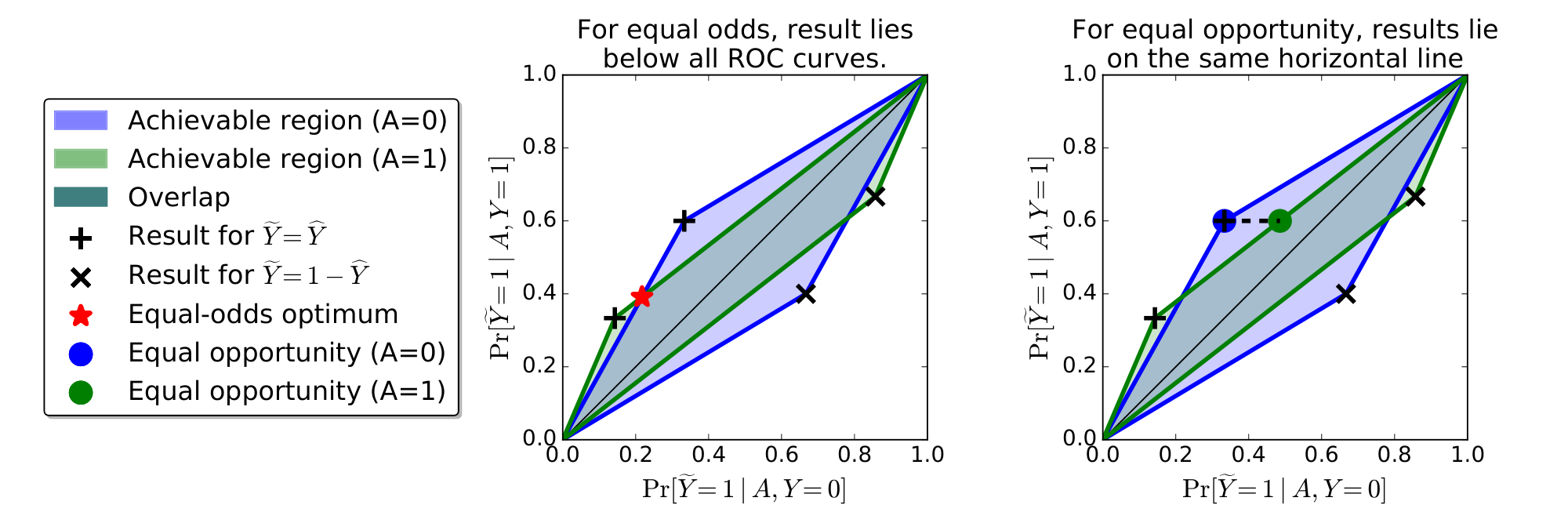
Our next lemma shows that $P_0(\widehat{Y})$ and $P_1(\widehat{Y})$ characterize exactly the trade-offs between false positives and true positives that we can achieve with any derived classifier. The polytopes are visualized in Figure 1.

########## {caption="Lemma 2"}

A predictor $\widetilde{Y}$ is derived if and only if for all $a\in{0, 1}, $ we have $\gamma_a(\widetilde{Y})\in P_a(\widehat{Y}).$

Proof: Since a derived predictor $\widetilde{Y}$ can only depend on $(\widehat{Y}, A)$ and these variables are binary, the predictor $\widetilde{Y}$ is completely described by four parameters in $[0, 1]$ corresponding to the probabilities $\Pr\left{\widetilde{Y} =1 \mid \widehat{Y}= \widehat{y}, A=a\right}$ for $\widehat{y}, a\in {0, 1}.$ Each of these parameter choices leads to one of the points in $P_a(\widehat{Y})$ and every point in the convex hull can be achieved by some parameter setting.

Combining Lemma 1 with Lemma 2, we see that the following optimization problem gives the optimal derived predictor with equalized odds:

$ \begin{align} \min_{\widetilde{Y}}\quad & \mathbb{E}\ell(\widetilde{Y}, Y)\ \mathrm{s.t.}\quad&\forall a\in {0, 1}: \gamma_a(\widetilde{Y})\in P_a(\widehat{Y})\quad \tag{\text{derived}}\ & \gamma_0(\widetilde{Y}) = \gamma_1(\widetilde{Y})\tag{\text{equalized odds}} \end{align}\tag{2} $

Figure 1 gives a simple geometric picture for the solution of the linear program whose guarantees are summarized next.

########## {caption="Proposition 3"}

The optimization problem Equation 2 is a linear program in four variables whose coefficients can be computed from the joint distribution of $(\widehat{Y}, A, Y).$ Moreover, its solution is an optimal equalized odds predictor derived from $\widehat{Y}$ and $A.$

Proof of Proposition 3: The second claim follows by combining Lemma 1 with Lemma 2. To argue the first claim, we saw in the proof of Lemma 2 that a derived predictor is specified by four parameters and the constraint region is an intersection of two-dimensional linear constraints. It remains to show that the objective function is a linear function in these parameters. Writing out the objective, we have

$ \mathbb{E}\left[\ell(\widetilde{Y}, Y)\right] = \sum_{y, y'\in {0, 1}} \ell(y, y')\Pr\left{\widetilde{Y}=y', Y=y\right}, . $

Further,

$ \begin{align*} \Pr\left{\widetilde{Y}=y', Y=y\right} & = \Pr\left{\widetilde{Y}=y', Y=y\mid \widetilde{Y}= \widehat{Y}\right}\Pr\left{\widetilde{Y}= \widehat{Y}\right}\ & \quad + \Pr\left{\widetilde{Y}=y', Y=y\mid \widetilde{Y}\neq \widehat{Y}\right}\Pr\left{\widetilde{Y}\neq \widehat{Y}\right}\ & = \Pr\left{\widehat{Y}=y', Y=y\right}\Pr\left{\widetilde{Y}= \widehat{Y}\right}

• \Pr\left{\widehat{Y}=1-y', Y=y\right}\Pr\left{\widetilde{Y}\neq \widehat{Y}\right}, . \end{align*} $

All probabilities in the last line that do not involve $\widetilde{Y}$ can be computed from the joint distribution. The probabilities that do involve $\widetilde{Y}$ are each a linear function of the parameters that specify $\widetilde{Y}.$

The corresponding optimization problem for equation opportunity is the same except that it has a weaker constraint $\gamma_0(\widetilde{Y})_2 = \gamma_1(\widetilde{Y})_2$. The proof is analogous to that of Proposition 3. Figure 1 explains the solution geometrically.

4.2 Deriving from a score function

We now consider deriving non-discriminating predictors from a real valued score $R\in[0, 1]$. The motivation is that in many realistic scenarios (such as FICO scores), the data are summarized by a one-dimensional score function and a decision is made based on the score, typically by thresholding it. Since a continuous statistic can carry more information than a binary outcome $Y$, we can hope to achieve higher utility when working with $R$ directly, rather then with a binary predictor $\widehat{Y}$.

A "protected attribute blind" way of deriving a binary predictor from $R$ would be to threshold it, i.e. using $\widehat{Y}= \mathbb{I}\left{R>t\right}$. If $R$ satisfied equalized odds, then so will such a predictor, and the optimal threshold should be chosen to balance false positive and false negatives so as to minimize the expected loss. When $R$ does not already satisfy equalized odds, we might need to use different thresholds for different values of $A$ (different protected groups), i.e. $\widetilde{Y}= \mathbb{I}\left{R>t_A\right}$. As we will see, even this might not be sufficient, and we might need to introduce additional randomness as in the preceding section.

Central to our study is the ROC (Receiver Operator Characteristic) curve of the score, which captures the false positive and true positive (equivalently, false negative) rates at different thresholds. These are curves in a two dimensional plane, where the horizontal axes is the false positive rate of a predictor and the vertical axes is the true positive rate. As discussed in the previous section, equalized odds can be stated as requiring the true positive and false positive rates, ($\Pr\left{\widehat{Y}=1 \mid Y=0, A=a\right}, \Pr\left{\widehat{Y}=1 \mid Y=1, A=a\right}$), agree between different values of $a$ of the protected attribute. That is, that for all values of the protected attribute, the conditional behavior of the predictor is at exactly the same point in this space. We will therefor consider the $A$-conditional ROC curves

$ C_a(t)\stackrel{\small \mathrm{def}}{=}\left(\Pr\left{\widehat{R} > t \mid A=a, Y=0\right}, \Pr\left{\widehat{R} > t \mid A=a, Y=1\right}\right). $

Since the ROC curves exactly specify the conditional distributions $R|A, Y$, a score function obeys equalized odds if and only if the ROC curves for all values of the protected attribute agree, that is $C_a(t)=C_{a'}(t)$ for all values of $a$ and $t$. In this case, any thresholding of $R$ yields an equalized odds predictor (all protected groups are at the same point on the curve, and the same point in false/true-positive plane).

When the ROC curves do not agree, we might choose different thresholds $t_a$ for the different protected groups. This yields different points on each $A$-conditional ROC curve. For the resulting predictor to satisfy equalized odds, these must be at the same point in the false/true-positive plane. This is possible only at points where all $A$-conditional ROC curves intersect. But the ROC curves might not all intersect except at the trivial endpoints, and even if they do, their point of intersection might represent a poor tradeoff between false positive and false negatives.

As with the case of correcting a binary predictor, we can use randomization to fill the span of possible derived predictors and allow for significant intersection in the false/true-positive plane. In particular, for every protected group $a$, consider the convex hull of the image of the conditional ROC curve:

$ D_a \stackrel{\small \mathrm{def}}{=} \mathrm{convhull}\left{ C_a(t)\colon t\in[0, 1]\right}\tag{3} $

The definition of $D_a$ is analogous to the polytope $P_a$ in the previous section, except that here we do not consider points below the main diagonal (line from $(0, 0)$ to $(1, 1)$), which are worse than "random guessing" and hence never desirable for any reasonable loss function.

Deriving an optimal equalized odds threshold predictor.

Any point in the convex hull $D_a$ represents the false/true positive rates, conditioned on $A=a$, of a randomized derived predictor based on $R$. In particular, since the space is only two-dimensional, such a predictor $\widetilde Y$ can always be taken to be a mixture of two threshold predictors (corresponding to the convex hull of two points on the ROC curve). Conditional on $A=a, $ the predictor $\widetilde Y$ behaves as

$ \widetilde{Y} = \mathbb{I}\left{R>T_a\right}, , $

where $T_a$ is a randomized threshold assuming the value $\underline{t}_a$ with probability $\underline{p}_a$ and the value $\overline{t}_a$ with probability $\overline{p}_a$. In other words, to construct an equalized odds predictor, we should choose a point in the intersection of these convex hulls, $\gamma=(\gamma_0, \gamma_1) \in \cap_a D_a$, and then for each protected group realize the true/false-positive rates $\gamma$ with a (possible randomized) predictor $\widetilde{Y}|(A=a) = \mathbb{I}\left{R>T_a\right}$ resulting in the predictor $\widetilde{Y} = \Pr \mathbb{I}\left{R>T_A\right}$. For each group $a$, we either use a fixed threshold $T_a=t_a$ or a mixture of two thresholds $\underline{t}_a<\overline{t}_a$. In the latter case, if $A=a$ and $R<\underline{t}_a$ we always set $\widetilde{Y}=0$, if $R>\overline{t}_a$ we always set $\widetilde{Y}=1$, but if $\underline{t}_a<R<\overline{t}_a$, we flip a coin and set $\widetilde{Y}=1$ with probability $\underline{p}_a$.

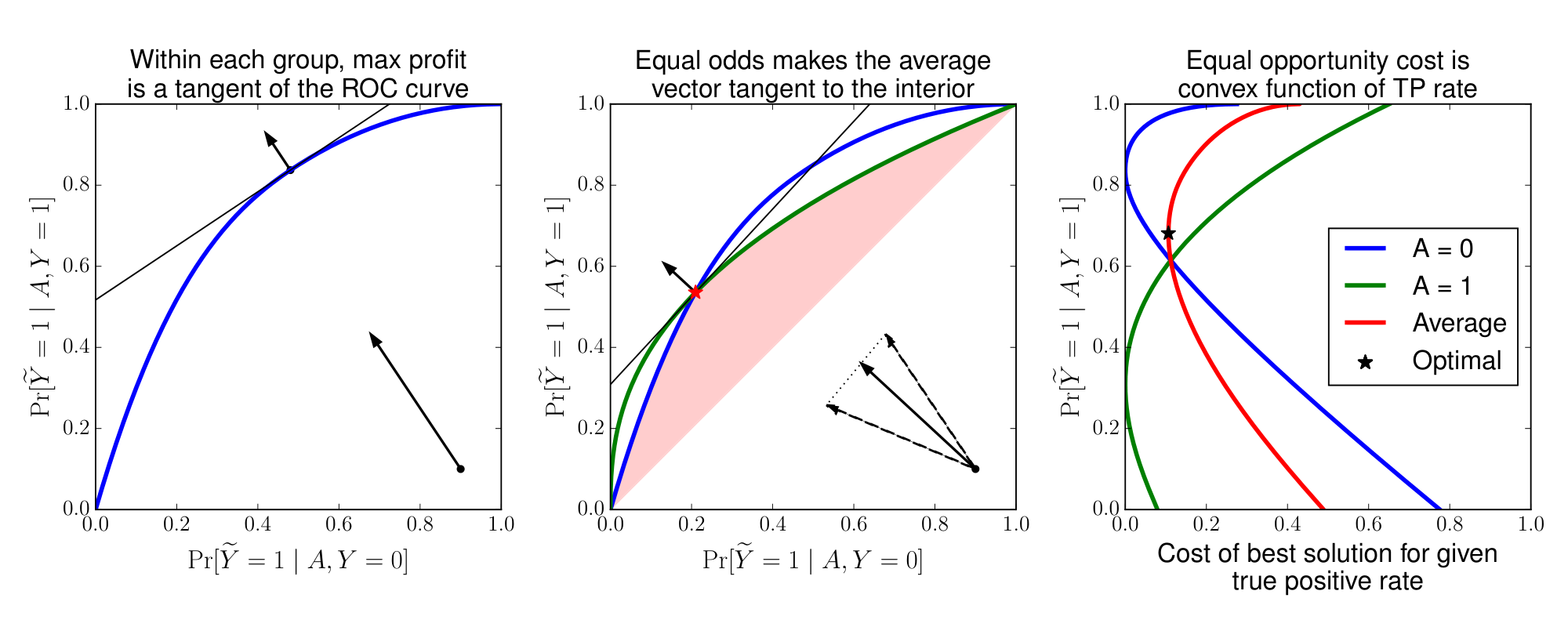
The feasible set of false/true positive rates of possible equalized odds predictors is thus the intersection of the areas under the $A$-conditional ROC curves, and above the main diagonal (see Figure 2). Since for any loss function the optimal false/true-positive rate will always be on the upper-left boundary of this feasible set, this is effectively the ROC curve of the equalized odds predictors. This ROC curve is the pointwise minimum of all $A$-conditional ROC curves. The performance of an equalized odds predictor is thus determined by the minimum performance among all protected groups. Said differently, requiring equalized odds incentivizes the learner to build good predictors for all classes. For a given loss function, finding the optimal tradeoff amounts to optimizing (assuming w.l.o.g. $\ell(0, 0)=\ell(1, 1)=0$):

$ \min_{\forall a\colon \gamma\in D_a} \gamma_0\ell(1, 0)+(1-\gamma_1)\ell(0, 1)\tag{4} $

This is no longer a linear program, since $D_a$ are not polytopes, or at least are not specified as such. Nevertheless, Equation 4 can be efficiently optimized numerically using ternary search.

Deriving an optimal equal opportunity threshold predictor.

The construction follows the same approach except that there is one fewer constraint. We only need to find points on the conditional ROC curves that have the same true positive rates in both groups. Assuming continuity of the conditional ROC curves, this means we can always find points on the boundary of the conditional ROC curves. In this case, no randomization is necessary. The optimal solution corresponds to two deterministic thresholds, one for each group. As before, the optimization problem can be solved efficiently using ternary search over the target true positive value. Here we use, as Figure 2 illustrates, that the cost of the best solution is convex as a function of its true positive rate.

5. Bayes optimal predictors

Section Summary: This section explains how to create the best possible fair classifiers that avoid discrimination based on protected attributes like race or gender, building on the idea of a "Bayes optimal regressor," which is essentially the most accurate way to predict an outcome from data. It shows that an ideal fair classifier, one that treats groups equally in terms of prediction accuracy, can be derived by simply applying a threshold to this optimal regressor along with the protected attribute. Additionally, it demonstrates that even if you use a slightly imperfect regressor, the resulting fair classifier remains nearly as good, with the shortfall measurable by a specific distance metric, supporting a two-step process of first building an unbiased predictor and then adjusting it for fairness.

In this section, we develop the theory a theory for non-discriminating Bayes optimal classification. We will first show that a Bayes optimal equalized odds predictor can be obtained as an derived threshold predictor of the Bayes optimal regressor. Second, we quantify the loss of deriving an equalized odds predictor based on a regressor that deviates from the Bayes optimal regressor. This can be used to justify the approach of first training classifiers without any fairness constraint, and then deriving an equalized odds predictor in a second step.

########## {caption="Bayes optimal regressor" type="Definition"}

Given random variables $(X, A)$ and a target variable $Y, $ the Bayes optimal regressor is $R=\arg\min_{r(x, a)}\mathbb{E}\left[(Y-r(X, A))^2\right]=r^*(X, A)$ with $r^*(x, a) = \mathbb{E}[Y \mid X=x, A=a].$

The Bayes optimal classifier, for any proper loss, is then a threshold predictor of $R, $ where the threshold depends on the loss function (see, e.g., [14]). We will extend this result to the case where we additionally ask the classifier to satisfy an oblivious property, such as our non-discrimination properties.

########## {caption="Proposition 4"}

For any source distribution over $(Y, X, A)$ with Bayes optimal regressor $R(X, A)$, any loss function, and any oblivious property $C$, there exists a predictor $Y^*(R, A)$ such that:

1. $Y^*$ is an optimal predictor satisfying $C$. That is, $\mathbb{E}\ell(Y^*, Y)\leqslant \mathbb{E}\ell(\widehat{Y}, Y)$ for any predictor $\widehat{Y}(X, A)$ which satisfies $C$.
2. $Y^*$ is derived from $(R, A).$

Proof: Consider an arbitrary classifier $\widehat{Y}$ on the attributes $(X, A)$, defined by a (possibly randomized) function $\widehat{Y}=f(X, A).$ Given $(R=r, A=a)$, we can draw a fresh $X'$ from the distribution $(X \mid R=r, A=a)$, and set $Y^* = f(X', a)$. This satisfies (2). Moreover, since $Y$ is binary with expectation $R$, $Y$ is independent of $X$ conditioned on $(R, A)$. Hence $(Y, X, R, A)$ and $(Y, X', R, A)$ have identical distributions, so $(Y^*, A, Y)$ and $(\widehat{Y}, A, Y)$ also have identical distributions. This implies $Y^*$ satisfies (1) as desired.

########## {caption="Corollary 5: Optimality characterization"}

An optimal equalized odds predictor can be derived from the Bayes optimal regressor $R$ and the protected attribute $A.$ The same is true for an optimal equal opportunity predictor.

5.1 Near optimality

We can furthermore show that if we can approximate the (unconstrained) Bayes optimal regressor well enough, then we can also construct a nearly optimal non-discriminating classifier.

To state the result, we introduce the following distance measure on random variables.

########## {type="Definition"}

We define the conditional Kolmogorov distance between two random variables $R, R'\in[0, 1]$ in the same probability space as $A$ and $Y$ as:

$ d_{\mathrm{K}}(R, R')\stackrel{\small \mathrm{def}}{=} \max_{a, y\in{0, 1}} \sup_{t\in[0, 1]} \left|\Pr\left{R > t\mid A=a, Y=y\right}

• \Pr\left{R' > t\mid A=a, Y=y\right} \right|, . $

Without the conditioning on $A$ and $Y, $ this definition coincides with the standard Kolmogorov distance. Closeness in Kolmogorov distance is a rather weak requirement. We need the slightly stronger condition that the Kolmogorov distance is small for each of the four conditionings on $A$ and $Y.$ This captures the distance between the restricted ROC curves, as formalized next.

########## {caption="Lemma 6"}

Let $R, R'\in[0, 1]$ be random variables in the same probability space as $A$ and $Y.$ Then, for any point $p$ on a restricted ROC curve of $R, $ there is a point $q$ on the corresponding restricted ROC curve of $R'$ such that $|p-q|_2 \leqslant\sqrt{2}\cdot d_K(R, R').$

Proof: Assume the point $p$ is achieved by thresholding $R$ at $t\in[0, 1].$ Let $q$ be the point on the ROC curve achieved by thresholding $R'$ at the same threshold $t'.$ After applying the definition to bound the distance in each coordinate, the claim follows from Pythagoras' theorem.

We can now show that an equalized odds predictor derived from a nearly optimal regressor is still nearly optimal among all equal odds predictors, while quantifying the loss in terms of the conditional Kolmogorov distance.

########## {caption="Theorem 7: Near optimality"}

Assume that $\ell$ is a bounded loss function, and let $\widehat{R}\in[0, 1]$ be an arbitrary random variable. Then, there is an optimal equalized odds predictor $Y^*$ and an equalized odds predictor $\widetilde{Y}$ derived from $(\widehat{R}, A)$ such that

$ \mathbb{E}\ell(\widetilde{Y}, Y)\leqslant \mathbb{E}\ell(Y^*, Y) + 2\sqrt{2}\cdot d_{\mathrm{K}}(\widehat{R}, R^*), , $

where $R^*$ is the Bayes optimal regressor. The same claim is true for equal opportunity.

Proof of Theorem 5.6: We prove the claim for equalized odds. The case of equal opportunity is analogous.

Fix the loss function $\ell$ and the regressor $\widehat{R}.$ Take $Y^*$ to be the predictor derived from the Bayes optimal regressor $R^*$ and $A.$ By Corollary 5, we know that this is an optimal equalized odds predictor as required by the lemma. It remains to construct a derived equalized odds predictor $\widetilde{Y}$ and relate its loss to that of $Y^*.$

Recall the optimization problem for defining the optimal derived equalized odds predictor. Let $\widehat D_a$ be the constraint region defined by $\widehat{R}.$ Likewise, let $D_a^*$ be the constraint region under $R^*.$ The optimal classifier $Y^*$ corresponds to a point $p^*\in D_0^*\cap D_1^*.$ As a consequence of Lemma 6, we can find (not necessarily identical) points $q_0\in \widehat D_0$ and $q_1\in \widehat D_1$ such that for all $a\in{0, 1}, $

$ |p^*-q_a|2 \leqslant \sqrt{2}\cdot d{\mathrm{K}}(\widehat{R}, R^*), . $

We claim that this means we can also find a feasible point $q\in \widehat D_0\cap \widehat D_1$ such that

$ |p^*-q|2 \leqslant 2\cdot d{\mathrm{K}}(\widehat{R}, R^*), . $

To see this, assume without loss of generality that the first coordinate of $q_1$ is greater than the first coordinate of $q_0, $ and that all points $p^*, q_0, q_1$ lie above the main diagonal. By definition of $\widehat D_1, $ we know that the entire line segment $L_1$ from $(0, 0)$ to $q_1$ is contained in $\widehat D_1.$ Similarly, the entire line segment~ $L_0$ between $q_0$ and $(1, 1)$ is contained in $\widehat D_0.$ Now, take $q\in L_0\cap L_1.$ By construction, $q\in \widehat D_0\cap\widehat D_1$ defines a classifier $\widetilde{Y}$ derived from $\widehat{R}$ and $A.$ Moreover,

$ |p^*-q|_2^2 \leqslant |p^*-q_0|_2^2 + |p^*-q_0|2^2 \leqslant 4\cdot d{\mathrm{K}}(\widehat{R}, R^*)^2, . $

Finally, by assumption on the loss function, there is a vector $v$ with $|v|_2 \leqslant\sqrt{2}$ such that $\mathbb{E}\ell(\widetilde{Y}, Y)=\langle v, q\rangle$ and $\mathbb{E}\ell(Y^*, Y)=\langle v, p^*\rangle.$ Applying Cauchy-Schwarz,

$ \mathbb{E}\ell(\widetilde{Y}, Y)- \mathbb{E}\ell(Y^*, Y) = \langle v, q-p^*\rangle \leqslant |v|_2\cdot|q-p^*|2 \leqslant 2\sqrt{2}\cdot d{\mathrm{K}}(\widehat{R}, R^*), . $

This completes the proof.

6. Oblivious identifiability of discrimination

Section Summary: This section explores why "black box" tests for discrimination in predictive models, which only examine scores, protected attributes like race, and outcomes like loan repayment, cannot always pinpoint true unfairness. It presents two contrasting scenarios: one where a model's strong performance relies on proxies for the protected attribute, leading to biased profiling, and another where the model uses a legitimate feature correlated with the protected attribute, appearing fair but still violating fairness criteria like equalized odds. Despite their different implications for discrimination, these scenarios produce identical data patterns, making it impossible for any such test to distinguish between them and reliably judge a model's fairness.

Before turning to analyzing data, we pause to consider to what extent "black box" oblivious tests like ours can identify discriminatory predictions. To shed light on this issue, we introduce two possible scenarios for the dependency structure of the score, the target and the protected attribute. We will argue that while these two scenarios can have fundamentally different interpretations from the point of view of fairness, they can be indistinguishable from their joint distribution. In particular, no oblivious test can resolve which of the two scenarios applies.

Scenario I

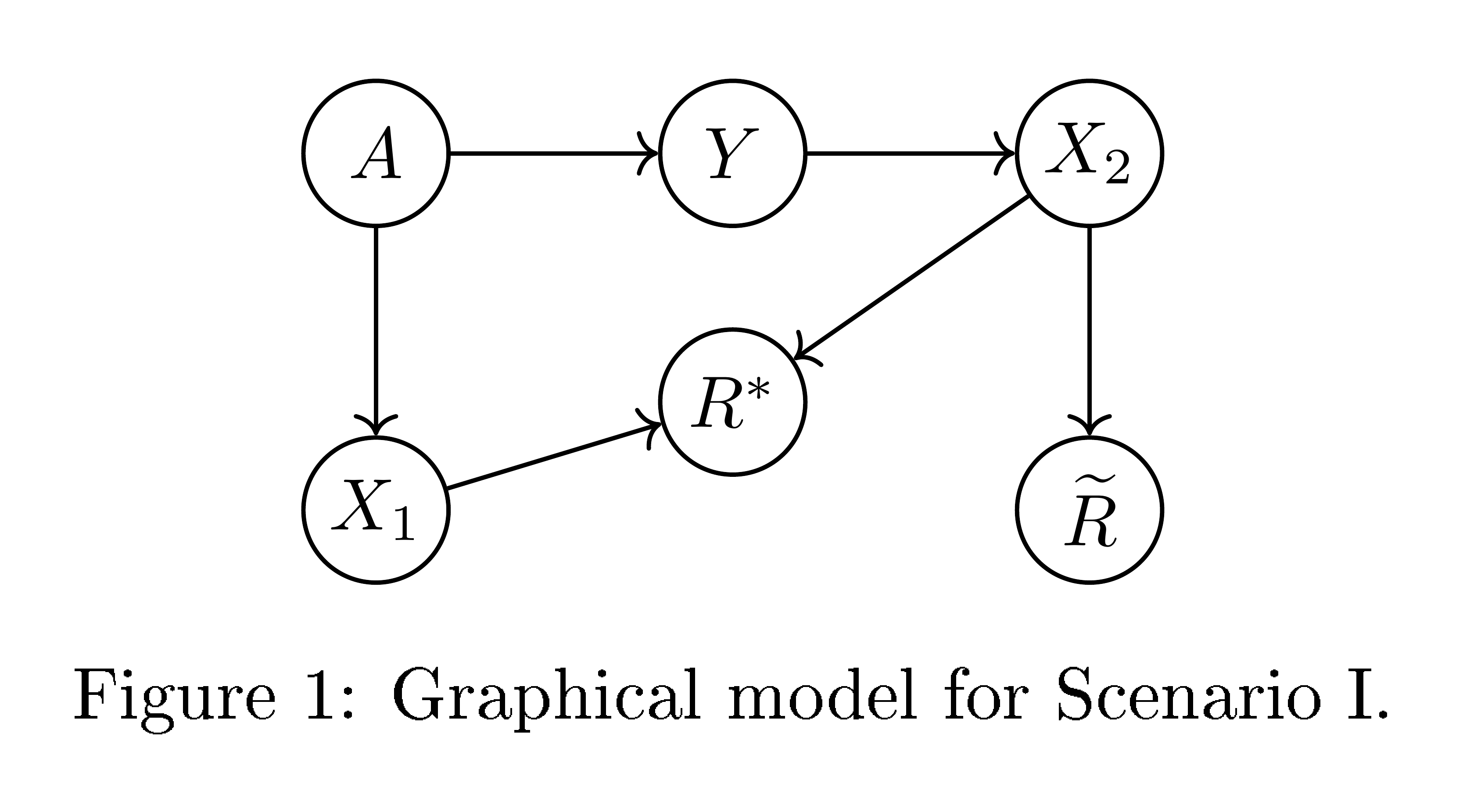
Consider the dependency structure depicted in Figure 4. Here, $X_1$ is a feature highly (even deterministically) correlated with the protected attribute $A$, but independent of the target $Y$ given $A$. For example, $X_1$ might be "languages spoken at home" or "great great grandfather's profession". The target $Y$ has a statistical correlation with the protected attribute. There's a second real-valued feature $X_2$ correlated with $Y$, but only related to $A$ through $Y$. For example, $X_2$ might capture an applicant's driving record if applying for insurance, financial activity if applying for a loan, or criminal history in criminal justice situations. An intuitively "fair" predictor here is to use only the feature $X_2$ through the score $\widetilde{R} = X_2$. The score $\widetilde{R}$ satisfies equalized odds, since $X_2$ and $A$ are independent conditional on $Y$. Because of the statistical correlation between $A$ and $Y$, a better statistical predictor, with greater power, can be obtained by taking into account also the protected attribute $A$, or perhaps its surrogate $X_1$. The statistically optimal predictor would have the form $R^*=r^*_{I}(X_2, X_1)$, biasing the score according to the protected attribute $A$. The score $R^*$ does not satisfy equalized odds, and in a sense seems to be "profiling" based on $A.$

Scenario II

Now consider the dependency structure depicted in Figure 5. Here $X_3$ is a feature, e.g. "wealth" or "annual income", correlated with the protected attribute $A$ and directly predictive of the target $Y$. That is, in this model, the probability of paying back of a loan is just a function of an individual's wealth, independent of their race. Using $X_3$ on its own as a predictor, e.g. using the score $R^*=X_3$, does not naturally seem directly discriminatory. However, as can be seen from the dependency structure, this score does not satisfy equalized odds. We can correct it to satisfy equalized odds and consider the optimal non-discriminating predictor $\widetilde{R}= \widetilde{r}_{II}(X_3, A)$ that does satisfy equalized odds. If $A$ and $X_3$, and thus $A$ and $Y$, are positively correlated, then $\widetilde{R}$ would depend inversely on $A$ (see numerical construction below), introducing a form of "corrective discrimination", so as to make $\widetilde{R}$ is independent of $A$ given $Y$ (as is required by equalized odds).

6.1 Unidentifiability

The above two scenarios seem rather different. The optimal score $R^*$ is in one case based directly on $A$ or its surrogate, and in another only on a directly predictive feature, but this is not apparent by considering the equalized odds criterion, suggesting a possible shortcoming of equalized odds. In fact, as we will now see, the two scenarios are indistinguishable using any oblivious test. That is, no test based only on the target labels, the protected attribute and the score would give different indications for the optimal score $R^*$ in the two scenarios. If it were judged unfair in one scenario, it would also be judged unfair in the other.

We will show this by constructing specific instantiations of the two scenarios where the joint distributions over $(Y, A, R^*, \widetilde{R})$ are identical. The scenarios are thus unidentifiable based only on these joint distributions.

We will consider binary targets and protected attributes taking values in $A, Y\in{-1, 1}$ and real valued features. We deviate from our convention of ${0, 1}$-values only to simplify the resulting expressions. In Scenario I, let:

• $\Pr\left{A=1\right}=1/2$, and $X_1=A$
• $Y$ follows a logistic model parametrized based on $A$: $\Pr\left{Y=y\mid A=a\right} = \frac1{1+\exp(-2ay)}, $
• $X_2$ is Gaussian with mean $Y$: $X_2=Y+{\mathcal N}(0, 1)$
• Optimal unconstrained and equalized odds scores are given by: $R^*=X_1 + X_2=A + X_2, $ and $\widetilde{R}=X_2$

In Scenario II, let:

• $\Pr\left{A=1\right}=1/2$.
• $X_3$ conditional on $A=a$ is a mixture of two Gaussians: ${\mathcal N}(a+1, 1)$ with weight $\frac1{1+\exp(-2a)}$ and ${\mathcal N}(a-1, 1)$ with weight $\frac1{1+\exp(2a)}.$
• $Y$ follows a logistic model parametrized based on $X_3$: $\Pr\left{Y=y\mid X_3=x_3\right}= \frac1{1+\exp(-2yx_3)}.$
• Optimal unconstrained and equalized odds scores are given by: $R^* = X_3, $ and $\widetilde{R}= X_3-A$

The following proposition establishes the equivalence between the scenarios and the optimality of the scores (proof at end of section):

########## {caption="Proposition 8"}

The joint distributions of $(Y, A, R^*, \widetilde{R})$ are identical in the above two scenarios. Moreover, $R^*$ and $\widetilde{R}$ are optimal unconstrained and equalized odds scores respectively, in that their ROC curves are optimal and for any loss function an optimal (unconstrained or equalized odds) classifier can be derived from them by thresholding.

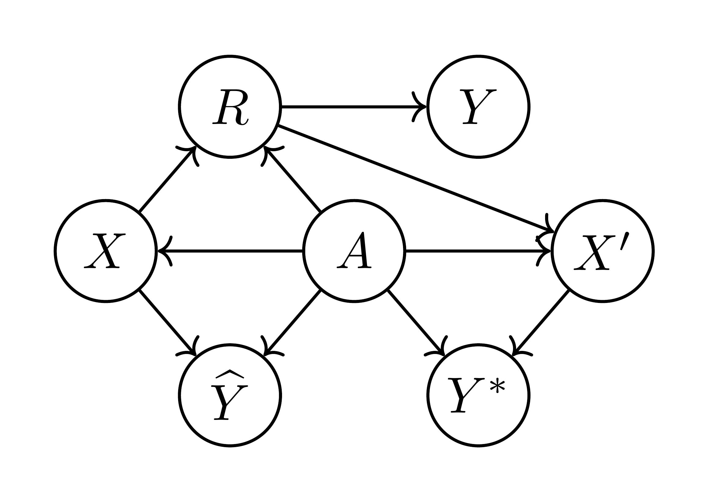
Not only can an oblivious test (based only on $(Y, A, R)$) not distinguish between the two scenarios, but even having access to the features is not of much help. Suppose we have access to all three feature, i.e. to a joint distribution over $(Y, A, X_1, X_2, X_3)$ —since the distributions over $(Y, A, R^*, \widetilde{R})$ agree, we can construct such a joint distribution with $X_2= \widetilde{R}$ and $X_3= \widetilde{R}$. The features are correlated with each other, with $X_3=X_1+X_2$. Without attaching meaning to the features or making causal assumptions about them, we do not gain any further insight on the two scores. In particular, both causal structures depicted in Figure 6 are possible.

6.2 Comparison of different oblivious measures

It is interesting to consider how different oblivious measures apply to the scores $\widetilde{R}$ and $R^*$ in these two scenarios.

As discussed in Section 4.2, a score satisfies equalized odds iff the conditional ROC curves agree for both values of $A$, which we refer to as having identical ROC curves.

########## {caption="Identical ROC Curves" type="Definition"}

We say that a score $R$ has identical conditional ROC curves if $C_a(t)=C_{a'}(t)$ for all groups of $a, a'$ and all $t\in\mathbb{R}$.

In particular, this property is achieved by an equalized odds score $\widetilde{R}$. Within each protected group, i.e. for each value $A=a$, the score $R^*$ differs from $\widetilde{R}$ by a fixed monotone transformation, namely an additive shift $R^*= \widetilde{R}+A$. Consider a derived threshold predictor $\widehat{Y}(\widetilde{R})= \mathbb{I}\left{\widetilde{R}>t\right}$ based on $\widetilde{R}$. Any such predictor obeys equalized odds. We can also derive the same predictor deterministically from $R^*$ and $A$ as $\widehat{Y}(R^*, A)= \mathbb{I}\left{R^*>t_A\right}$ where $t_A=t-A$. That is, in our particular example, $R^*$ is special in that optimal equalized odds predictors can be derived from it (and the protected attribute $A$) deterministically, without the need to introduce randomness as in Section 4.2. In terms of the $A$-conditional ROC curves, this happens because the images of the conditional ROC curves $C_0$ and $C_1$ overlap, making it possible to choose points in the true/false-positive rate plane that are on both ROC curves. However, the same point on the conditional ROC curves correspond to different thresholds! Instead of $C_0(t)=C_1(t)$, for $R^*$ we have $C_0(t)=C_1(t-1)$. We refer to this property as "matching" conditional ROC curves:

########## {caption="Matching ROC curves" type="Definition"}

We say that a score $R$ has matching conditional ROC curves if the images of all $A$-conditional ROC curves are the same, i.e., for all groups $a, a', $ $\left{ C_a(t) \colon t\in\mathbb{R} \right} = \left{ C_{a'}(t) \colon t\in\mathbb{R} \right}.$

Having matching conditional ROC curves corresponds to being deterministically correctable to be non-discriminating: If a predictor $R$ has matching conditional ROC curves, then for any loss function the optimal equalized odds derived predictor is a deterministic function of $R$ and $A$. But as our examples show, having matching ROC curves does not at all mean the score is itself non-discriminatory: it can be biased according to $A$, and a (deterministic) correction might be necessary in order to ensure equalized odds.

Having identical or matching ROC curves are properties of the conditional distribution $R|Y, A$, also referred to as "model errors". Oblivious measures can also depend on the conditional distribution $Y|R, A$, also referred to as "target population errors". In particular, one might consider the following property:

########## {caption="Matching frequencies" type="Definition"}

We say that a score $R$ has matching conditional frequencies, if for all groups $a, a'$ and all scores $t, $ we have

$ \Pr\left{Y=1\mid R=t, A=a\right} = \Pr\left{Y=1\mid R=t, A=a'\right}, . $

Matching conditional frequencies state that at a given score, both groups have the same probability of being labeled positive. The definition can also be phrased as requiring that the conditional distribution $Y|R, A$ be independent of $A$. In other words, having matching conditional frequencies is equivalent to $A$ and $Y$ being independent conditioned on $R$. The corresponding dependency structure is $Y-R-A$. That is, the score $R$ includes all possible information the protected attribute can provide on the target $Y$. Indeed having matching conditional frequencies means that the score is in a sense "optimally dependent" on the protected attribute $A$. Formally, for any loss function the optimal (unconstrained, possibly discriminatory) derived predictor $\widehat{Y}(R, A)$ would be a function of $R$ alone, since $R$ already includes all relevant information about $A$. In particular, an unconstrained optimal score, like $R^*$ in our constructions, would satisfy matching conditional frequencies. Having matching frequencies can therefore be seen as a property indicating utilizing the protected attribute for optimal predictive power, rather then protecting discrimination based on it.

It is also worth noting the similarity between matching frequencies and a binary predictor $\widehat{Y}$ having equal conditional precision, that is $\Pr\left{Y=1\mid \widehat{Y}= \widehat{y}, A=a\right} = \Pr\left{Y=1\mid \widehat{Y}= \widehat{y}, A=a'\right}$. Viewing $\widehat{Y}$ as a score that takes two possible values, the notions agree. But $R$ having matching conditional frequencies does not imply the threshold predictors $\widehat{Y}(R)= \mathbb{I}\left{R>t\right}$ will have matching precision—the conditional distributions $R|A$ might be different, and these are involved in marginalizing over $R>t$ and $R \leqslant t$.

To summarize, the properties of the scores in our scenarios are:

• $R^*$ is optimal based on the features and protected attribute, without any constraints.
• $\widetilde{R}$ is optimal among all equalized odds scores.
• $\widetilde R$ does satisfy equal odds, $R^*$ does not satisfy equal odds.
• $\widetilde R$ has identical (thus matching) ROC curves, $R^*$ has matching but non-identical ROC curves.
• $R^*$ has matching conditional frequencies, while $\widetilde{R}$ does not.

Proof of Proposition 6.1

First consider Scenario I. The score $\widetilde{R}=X_2$ obeys equalized odds due to the dependency structure. More broadly, if a score $R=f(X_2, X_1)$ obeys equalized odds, for some randomized function $f$, it cannot depend on $X_1$: conditioned on $Y$, $X_2$ is independent of $A=X_1$, and so any dependency of $f$ on $X_1$ would create a statistical dependency on $A=X_1$ (still conditioned on $Y$) which is not allowed. We can verify that $\Pr\left{Y=y\mid X_2=x_2\right} \propto \Pr\left{Y=y\right}\Pr\left{X_2=x_2\mid Y=y\right} \propto \exp(2y x_2)$ which is monotone in $X_2$, and so for any loss function we would just want to threshold $X_2$ and any function monotone in $X_2$ would make an optimal equalized odds predictor.

To obtain the optimal unconstrained score consider

$ \begin{align*} \Pr\left{Y=y\mid X_1=x_1, X_2=x_2\right} & \propto \Pr\left{A=x_1\right}\Pr\left{Y=y\mid A=x_1\right}\Pr\left{X_2=x_2\mid Y=y\right} \ &\propto\exp(2y(x_1+x_2)). \end{align*} $

That is, optimal classification only depends on $x_1+x_2$ and so $R^*=X_1+X_2$ is optimal.

Turning to scenario II, since $P(Y|X_3)$ is monotone in $X_3$, any monotone function of it is optimal (unconstrained), and the dependency structure implies its optimal even if we allow dependence on $A$. Furthermore, the conditional distribution $Y|X_3$ matched that of $Y|R^*$ from scenario I since again we have $\Pr\left{Y=y|X_3=x_3\right}\propto \exp(2 y x_3)$ by construction. Since we defined $R^*=X_3$, we have that the conditionals $R^*|Y$ match. We can also verify that by construction $X_3|A$ matches $R^*|A$ in scenario I. Since in scenario I, $R^*$ is optimal even dependent on $A$, we have that $A$ is independent of $Y$ conditioned on $R^*$, as in scenario II when we condition on $X_3=R^*$. This establishes the joint distribution over $(A, Y, R^*)$ is the same in both scenarios. Since $\widetilde{R}$ is the same deterministic function of $A$ and $R^*$ in both scenarios, we can further conclude the joint distributions over $A, Y, R^*$ and $\widetilde{R}$ are the same. Since equalized odds is an oblivious property, once these distributions match, if $\widetilde{R}$ obeys equalized odds in scenario I, it also obeys it in scenario II.

7. Case study: FICO scores

Section Summary: This case study explores fairness in FICO credit scores, which predict whether people will default on loans, using race as a protected factor based on 2003 data from over 300,000 individuals across Asian, white, Hispanic, and Black groups. Researchers compare loan approval thresholds under different rules: one maximizing lender profit without constraints, a race-blind approach using the same cutoff for everyone, and fairness measures like demographic parity (equal loan rates across races), equal opportunity (equal approval for non-defaulters), and equalized odds (equal rates for both defaulters and non-defaulters). Their findings show that fairness constraints produce thresholds between the profit-driven and strict equality options, revealing that FICO scores predict defaults less accurately for minority groups than for whites.

We examine various fairness measures in the context of FICO scores with the protected attribute of race. FICO scores are a proprietary classifier widely used in the United States to predict credit worthiness. Our FICO data is based on a sample of $301536$ TransUnion TransRisk scores from 2003 [15]. These scores, ranging from $300$ to $850$, try to predict credit risk; they form our score $R$. People were labeled as in default if they failed to pay a debt for at least $90$ days on at least one account in the ensuing 18-24 month period; this gives an outcome $Y$. Our protected attribute $A$ is race, which is restricted to four values: Asian, white non-Hispanic (labeled "white" in figures), Hispanic, and black. FICO scores are complicated proprietary classifiers based on features, like number of bank accounts kept, that could interact with culture—and hence race—in unfair ways.

A credit score cutoff of 620 is commonly used for prime-rate loans^1, which corresponds to an any-account default rate of 18%. Note that this measures default on any account TransUnion was aware of; it corresponds to a much lower ($\approx 2%$) chance of default on individual new loans. To illustrate the concepts, we use any-account default as our target $Y$ —a higher positive rate better illustrates the difference between equalized odds and equal opportunity.

We therefore consider the behavior of a lender who makes money on default rates below this, i.e., for whom whom false positives (giving loans to people that default on any account) is 82/18 as expensive as false negatives (not giving a loan to people that don't default). The lender thus wants to construct a predictor $\widehat{Y}$ that is optimal with respect to this asymmetric loss. A typical classifier will pick a threshold per group and set $\widehat{Y} = 1$ for people with FICO scores above the threshold for their group. Given the marginal distributions for each group (Figure 7), we can study the optimal profit-maximizing classifier under five different constraints on allowed predictors:

• Max profit has no fairness constraints, and will pick for each group the threshold that maximizes profit. This is the score at which 82% of people in that group do not default.
• Race blind requires the threshold to be the same for each group. Hence it will pick the single threshold at which 82% of people do not default overall, shown in Figure 8.
• Demographic parity picks for each group a threshold such that the fraction of group members that qualify for loans is the same.
• Equal opportunity picks for each group a threshold such that the fraction of non-defaulting group members that qualify for loans is the same.
• Equalized odds requires both the fraction of non-defaulters that qualify for loans and the fraction of defaulters that qualify for loans to be constant across groups. This cannot be achieved with a single threshold for each group, but requires randomization. There are many ways to do it; here, we pick two thresholds for each group, so above both thresholds people always qualify and between the thresholds people qualify with some probability.

We could generalize the above constraints to allow non-threshold classifiers, but we can show that each profit-maximizing classifier will use thresholds. As shown in Section 4, the optimal thresholds can be computed efficiently; the results are shown in Figure 9.

Our proposed fairness definitions give thresholds between those of max-profit/race-blind thresholds and of demographic parity.

Figure 10 plots the ROC curves for each group. It should be emphasized that differences in the ROC curve do not indicate differences in default behavior but rather differences in prediction accuracy—lower curves indicate FICO scores are less predictive for those populations. This demonstrates, as one should expect, that the majority (white) group is classified more accurately than minority groups, even over-represented minority groups like Asians.

The left side of Figure 11 shows the fraction of people that wouldn't default that would qualify for loans by the various metrics. Under max-profit and race-blind thresholds, we find that black people that would not default have a significantly harder time qualifying for loans than others. Under demographic parity, the situation is reversed.

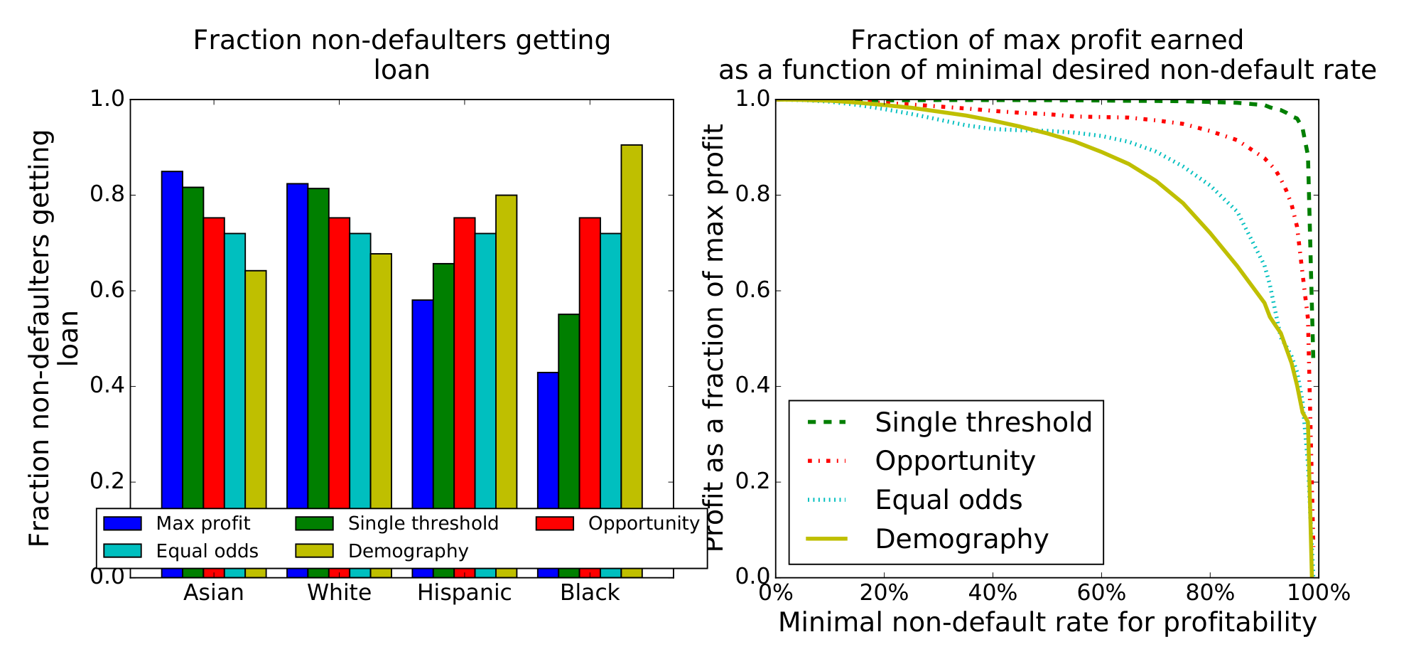
The right side of Figure 11 gives the profit achieved by each method, as a fraction of the max profit achievable. We show this as a function of the non-default rate above which loans are profitable (i.e. 82% in the other figures). At 82%, we find that a race blind threshold gets 99.3% of the maximal profit, equal opportunity gets 92.8%, equalized odds gets 80.2%, and demographic parity gets 69.8%. So equal opportunity fairness costs less than a quarter what demographic parity costs—and if the classifier improves, this would reduce further.

The difference between equal odds and equal opportunity is that under equal opportunity, the classifier can make use of its better accuracy among whites. Under equal odds this is viewed as unfair, since it means that white people who wouldn't pay their loans have a harder time getting them than minorities who wouldn't pay their loans. An equal odds classifier must classify everyone as poorly as the hardest group, which is why it costs over twice as much in this case. This also leads to more conservative lending, so it is slightly harder for non-defaulters of all groups to get loans.

The equal opportunity classifier does make it easier for defaulters to get loans if they are minorities, but the incentives are aligned properly. Under max profit, a small group may not be worth figuring out how to classify and so be treated poorly, since the classifier can't identify the qualified individuals. Under equal opportunity, such poorly-classified groups are instead treated better than well-classified groups. The cost is thus born by the company using the classifier, which can decide to invest in better classification, rather than the classified group, which cannot. Equalized odds gives a similar, but much stronger, incentive since the cost for a small group is not proportional to its size.

While race blindness achieves high profit, the fairness guarantee is quite weak. As with max profit, small groups may be classified poorly and so treated poorly, and the company has little incentive to improve the accuracy. Furthermore, when race is redundantly encoded, race blindness degenerates into max profit.

8. Conclusions

Section Summary: The authors propose a fairness measure for machine learning that fixes key flaws in traditional approaches like demographic parity while supporting the main aim of building more accurate predictors. They emphasize selecting reliable outcome data, such as loan default rates, and using the measure to spot potential biases for deeper investigation rather than claiming definitive proof of fairness or unfairness. The framework encourages better data collection and features to reduce bias, offers a simple post-processing fix that's efficient and privacy-friendly, and can involve shifting scores like affirmative action to ease the impact of uncertainty on protected groups.

We proposed a fairness measure that accomplishes two important desiderata. First, it remedies the main conceptual shortcomings of demographic parity as a fairness notion. Second, it is fully aligned with the central goal of supervised machine learning, that is, to build higher accuracy classifiers. In light of our results, we draw several conclusions aimed to help interpret and apply our framework effectively.

Choose reliable target variables.

Our notion requires access to observed outcomes such as default rates in the loan setting. This is precisely the same requirement that supervised learning generally has. The broad success of supervised learning demonstrates that this requirement is met in many important applications. That said, having access to reliable "labeled data" is not always possible. Moreover, the measurement of the target variable might in itself be unreliable or biased. Domain-specific scrutiny is required in defining and collecting a reliable target variable.

Measuring unfairness, rather than proving fairness.

Due to the limitations we described, satisfying our notion (or any other oblivious measure) should not be considered a conclusive proof of fairness. Similarly, violations of our condition are not meant to be a proof of unfairness. Rather we envision our framework as providing a reasonable way of discovering and measuring potential concerns that require further scrutiny. We believe that resolving fairness concerns is ultimately impossible without substantial domain-specific investigation. This realization echoes earlier findings in "Fairness through Awareness" [5] describing the task-specific nature of fairness.

Incentives.

Requiring equalized odds creates an incentive structure for the entity building the predictor that aligns well with achieving fairness. Achieving better prediction with equalized odds requires collecting features that more directly capture the target $Y$, unrelated to its correlation with the protected attribute. Deriving an equalized odds predictor from a score involves considering the pointwise minimum ROC curve among different protected groups, encouraging constructing of predictors that are accurate in all groups, e.g., by collecting data appropriately or basing prediction on features predictive in all groups.

When to use our post-processing step.

An important feature of our notion is that it can be achieved via a simple and efficient post-processing step. In fact, this step requires only aggregate information about the data and therefore could even be carried out in a privacy-preserving manner (formally, via Differential Privacy). In contrast, many other approaches require changing a usually complex machine learning training pipeline, or require access to raw data. Despite its simplicity, our post-processing step exhibits a strong optimality principle. If the underlying score was close to optimal, then the derived predictor will be close to optimal among all predictors satisfying our definition. However, this does not mean that the predictor is necessarily good in an absolute sense. It also does not mean that the loss compared to the original predictor is always small. An alternative to using our post-processing step is always to invest in better features and more data. Only when this is no longer an option, should our post-processing step be applied.

Predictive affirmative action.

In some situations, including Scenario II in Section 6, the equalized odds predictor can be thought of as introducing some sort of affirmative action: the optimally predictive score $R^*$ is shifted based on $A$. This shift compensates for the fact that, due to uncertainty, the score is in a sense more biased then the target label (roughly, $R^*$ is more correlated with $A$ then $Y$ is correlated with $A$). Informally speaking, our approach transfers the burden of uncertainty from the protected class to the decision maker. We believe this is a reasonable proposal, since it incentivizes the decision maker to invest additional resources toward building a better model.

References

Section Summary: This references section lists academic papers, government reports, and books primarily focused on the challenges of bias and fairness in big data and algorithmic systems. It includes early works on disparate impacts of big data analytics, such as those from the U.S. Executive Office of the President, and technical studies on building fair classifiers and representations to reduce discrimination in machine learning. Additional sources cover trade-offs between accuracy and fairness in risk assessments, as well as foundational texts on statistical inference and credit scoring practices.

[1] Solon Barocas and Andrew Selbst. Big data's disparate impact. California Law Review, 104, 2016.

[2] John Podesta, Penny Pritzker, Ernest J. Moniz, John Holdren, and Jefrey Zients. Big data: Seizing opportunities and preserving values. Executive Office of the President, May 2014.

[3] Big data: A report on algorithmic systems, opportunity, and civil rights. Executive Office of the President, May 2016.

[4] Dino Pedreshi, Salvatore Ruggieri, and Franco Turini. Discrimination-aware data mining. In Proc. $14$th ACM SIGKDD, 2008.

[5] Cynthia Dwork, Moritz Hardt, Toniann Pitassi, Omer Reingold, and Richard S. Zemel. Fairness through awareness. In Proc. ACM ITCS, pages 214–226, 2012.

[6] Andrea Romei and Salvatore Ruggieri. A multidisciplinary survey on discrimination analysis. The Knowledge Engineering Review, 29:582–638, 11 2014.

[7] T. Calders, F. Kamiran, and M. Pechenizkiy. Building classifiers with independency constraints. In In Proc. IEEE International Conference on Data Mining Workshops, pages 13–18, 2009.

[8] Indre Zliobaite. On the relation between accuracy and fairness in binary classification. CoRR, abs/1505.05723, 2015.

[9] Muhammad Bilal Zafar, Isabel Valera, Manuel Gomez Rodriguez, and Krishna P Gummadi. Learning fair classifiers. CoRR, abs:1507.05259, 2015.

[10] Richard S. Zemel, Yu Wu, Kevin Swersky, Toniann Pitassi, and Cynthia Dwork. Learning fair representations. In Proc. $30$th ICML, 2013.

[11] Christos Louizos, Kevin Swersky, Yujia Li, Max Welling, and Richard S. Zemel. The variational fair autoencoder. CoRR, abs/1511.00830, 2015.

[12] Michael Feldman, Sorelle A. Friedler, John Moeller, Carlos Scheidegger, and Suresh Venkatasubramanian. Certifying and removing disparate impact. In Proc. $21$st ACM SIGKDD, pages 259–268. ACM, 2015.

[13] Jon M. Kleinberg, Sendhil Mullainathan, and Manish Raghavan. Inherent trade-offs in the fair determination of risk scores. CoRR, abs/1609.05807, 2016.

[14] Larry Wasserman. All of Statistics: A Concise Course in Statistical Inference. Springer, 2010.

[15] US Federal Reserve. Report to the congress on credit scoring and its effects on the availability and affordability of credit, 2007.