Discrete State Diffusion Models: A Sample Complexity Perspective
Aadithya Srikanth$^{}$, Mudit Gaur$^{}$, Vaneet Aggarwal
Purdue University, West Lafayette, IN
Correspondence: Aadithya Srikanth [email protected], Mudit Gaur [email protected], Vaneet Aggarwal [email protected]
Abstract
Diffusion models have demonstrated remarkable performance in generating high-dimensional samples across domains such as vision, language, and the sciences. Although continuous-state diffusion models have been extensively studied both empirically and theoretically, discrete-state diffusion models, essential for applications involving text, sequences, and combinatorial structures, remain significantly less understood from a theoretical standpoint. In particular, all existing analyses of discrete-state models assume score estimation error bounds without studying sample complexity results. In this work, we present a principled theoretical framework for discrete-state diffusion, providing the first sample complexity bound of $\widetilde{\mathcal{O}}(\epsilon^{-2})$. Our structured decomposition of the score estimation error into statistical, approximation, optimization, and clipping components offers critical insights into how discrete-state models can be trained efficiently. This analysis addresses a fundamental gap in the literature and establishes the theoretical tractability and practical relevance of discrete-state diffusion models.
$^*$ Equal contribution
Paper will be presented at AISTATS 2026
Executive Summary: Discrete-state diffusion models, a type of generative AI tool, excel at creating data like text, molecular structures, and sequences by gradually adding and then removing noise. While continuous-state versions—used for images and audio—have strong theoretical backing, discrete versions lag behind, especially in understanding how many training samples are truly needed to produce high-quality outputs. This gap matters now as discrete models power growing applications in natural language processing, drug discovery, and protein design, where inefficient training could waste resources or limit scalability in industries like pharmaceuticals and tech.
This paper aims to fill that gap by deriving the first rigorous bounds on sample complexity for training discrete-state diffusion models. It evaluates how many data samples suffice to train a neural network that estimates the model's "score function"—a key component for reversing the noise process—so the generated distribution matches the original within a small error margin, measured by KL divergence.
The authors develop a theoretical framework using continuous-time Markov chains to model the diffusion process on discrete spaces, like alphabets of size S in d dimensions. They decompose the score estimation error into four parts: approximation (how well the neural network represents the true score), statistical (from finite data), optimization (from imperfect training via stochastic gradient descent), and clipping (to keep outputs bounded). Analysis relies on standard assumptions, such as smooth losses and bounded data scores, over a training period up to time T, with neural networks of depth L and width W trained on n samples per time step. This setup draws from recent continuous-state results but adapts to discrete sparsity, ensuring bounds scale reasonably with data size N = S^d without full enumeration.
The core findings are: First, about 1/ε² samples (ignoring logs) are enough to generate samples ε-close to the target distribution in KL divergence, a rate optimal for mean estimation tasks and better than prior continuous-state bounds of 1/ε⁴ or 1/ε⁵. Second, approximation error drops to zero if network width exceeds (S-1)d, leveraging the discrete score's low effective dimension of d(S-1). Third, statistical and optimization errors each scale as roughly sqrt(log(1/γ)/n) times network size factors, combining to drive the overall 1/ε² rate under a mild landscape condition. Fourth, total steps needed for convergence grow as sqrt(S²/ε) times logs or linearly in d, far better than dimension-squared penalties in some earlier discrete analyses. Fifth, no early stopping is required if initial scores are bounded.
These results mean discrete diffusion models are not just empirically promising but theoretically efficient, requiring fewer samples than expected for reliable generation in high-stakes fields. They reduce risk in applications like molecule design, where poor samples could delay drug trials, and improve performance by quantifying trade-offs: wider networks eliminate approximation gaps but raise optimization costs, while more samples cut statistical error at the expense of data needs. Unlike prior work assuming perfect score estimates, this ties theory to practical neural training, confirming discrete models match continuous ones in sample efficiency without exponential dimension blowup.
Leaders should prioritize datasets of at least 1/ε² size for target accuracy ε, using networks wide enough to interpolate scores exactly, and allocate training budgets accordingly—e.g., for ε=0.01 in text generation, expect millions of samples but feasible with modern hardware. Trade-offs include deeper networks (higher L) worsening bounds slightly, so shallower ones may suit initial pilots. Next, validate via experiments on real datasets like proteins; if gaps emerge, refine with finite-width approximations.
Limitations include reliance on assumptions like bounded scores and a Polyak-Łojasiewicz condition for loss landscapes, which hold in overparameterized settings but may not in all nonconvex cases, plus ignoring full network depth scaling in practice. Confidence is high for the Õ(1/ε²) bound under these conditions, as it matches information-theoretic lower bounds, but readers should temper expectations for very unbalanced data distributions without further tweaks.
1. Introduction
Section Summary: Diffusion models have become popular for creating new data in fields like images, audio, and text by gradually adding noise to real samples and then learning to reverse the process to generate realistic ones. While much early work focused on continuous data like photos, there's growing interest in discrete data such as words or molecular structures, but previous studies left open questions about how many training samples are truly needed to make these models work well. This paper fills that gap by providing the first rigorous estimates of sample requirements for discrete diffusion models, breaking down the errors in estimating the key "score" function into parts like network limitations, data scarcity, training imperfections, and output constraints, ultimately showing that a manageable number of samples can produce generated data very close to the original distribution.
Diffusion Models ([1]) have gained significant attention lately due to their empirical success in various generative modeling tasks across computer vision and audio generation ([2, 3]), text generation ([4]), sequential data modeling ([5]), policy learning ([6]), life sciences ([7, 8, 9]), and biomedical image reconstruction ([10]). They model an unknown and unstructured distribution through forward and reverse stochastic processes. In the forward process, samples from the dataset are gradually corrupted to obtain a stationary distribution. In the reverse process, a well-defined noisy distribution is used as the initialization to iteratively produce samples that resemble the learnt distribution using the score function. Most of the earlier works have been on continuous-state diffusion models, where the data is defined on the Euclidean space $\mathcal{R}^d$, unlike the discrete data, which is defined on $\mathcal{S}^d$, where $\mathcal{S}$ is the discrete set of values each component can take and $d$ is the number of components or dimension of the data. Given the growing number of applications of generative AI with discrete data, such as text generation ([11]) and summarization ([12]), combinatorial optimization ([13]), molecule generation and drug discovery ([8]), protein and DNA sequence design [47, 14], and graph generation [15], there has been an increased interest in diffusion with discrete data. For a more complete review of related literature, one may refer to [16].
[17] initiated the theoretical study of score-based discrete-state diffusion models. They proposed a sampling algorithm for the hypercube ${0, 1}^d$, using uniformization under the Continuous Time Markov Chain (CTMC) framework to establish convergence guarantees and bounds on iteration complexity. [18] further extended this theory to a general state space, $[S]^d$, and proposed a discrete-time sampling algorithm for high-dimensional data. They provided KL convergence bounds centered on truncation, discretization, and score estimation error decomposition. [19] proposed a Lévy-type stochastic integral framework for the error analysis of discrete-state diffusion models. They implemented both $\tau$ leaping and uniformization algorithms and presented error bounds in KL divergence, the first for the $\tau$ leaping scheme. However, it is important to note that these error analyses were performed under the assumption of access to an $\epsilon_{score}$ -accurate score estimator. Prior works by [17], [18], and [19] laid the foundation for the theoretical study and analyzed iteration complexity, while the sample complexity is an unexplored topic. In this work, we bridge this gap by providing the first sample complexity bounds for discrete-state diffusion models, offering rigorous insight into the number of samples required to estimate the score function to within a desired accuracy. We perform a detailed analysis of the score estimation error bound $\epsilon_{score}$, which was simply assumed in earlier works.
Specifically, we seek an answer to the following question.
To the best of our knowledge, this work offers the first theoretical investigation into the sample complexity of discrete-state diffusion models. We introduce a recursive analytical framework that traces the optimization error incurred at each step of SGD, allowing us to quantify the effect of performing only a limited number of optimization steps when learning the discrete-state score. Our approach bounds the discrepancy between the empirical and expected loss directly over a finite hypothesis class, thereby bypassing complexity measures that scale poorly with network size. An essential component of our analysis is the application of the Polyak–Łojasiewicz (PL) condition (Assumption 1), which ensures a quadratic lower bound on the error and is crucial for regulating the overall error in score estimation.
We summarize our main contributions as follows:
- First sample complexity bounds for discrete-state diffusion models To the best of our knowledge, this is the first work to present rigorous sample complexity analyses under reasonable and practical assumptions for discrete-state diffusion models. We derive an order optimal bound of $\widetilde{\mathcal{O}}(\epsilon^{-2})$, and thus providing deeper insight into the sample efficiency of discrete-state diffusion. In particular we prove that $\widetilde{\mathcal{O}}(\epsilon^{-2})$ samples are enough for discrete-state diffusion models to generate samples from a distribution that is $\epsilon$-close to the target distribution in KL divergence.
- Principled error decomposition We propose a structured decomposition of the score estimation error into approximation, statistical, optimization, and clipping components, enabling the characterization of how each factor contributes to the overall sample complexity.
2. Related Work
Section Summary: Discrete-state diffusion models, which are like probabilistic chains that evolve in steps to generate data, began as simple Markov processes and were adapted into versions called D3PMs to mimic continuous models, though they mostly found use outside language tasks due to practical hurdles. These models provide ways to sample data but often lack flexibility and solid theoretical backing, with early continuous-time versions relying on rate matrices to reverse the process. While analysis of their accuracy lags behind continuous counterparts, recent studies have improved error bounds and sampling efficiency, and this work introduces a new sample complexity measure for discrete models that scales better than previous ones.
2.1 Discrete-state Diffusion Models
Discrete-state diffusion models were initially studied as discrete-time Markov chains, which train and sample the model at discrete time points. [20] first proposed Discrete Denoising Diffusion Probabilistic Models (D3PMs) as the discrete-state analog of the "mean predicting" DDPMs ([21]). These models were largely applied to fields other than language due to empirical challenges ([22]). Although these models offer various practical sampling algorithms, they lack flexibility and theoretical guarantees ([18]). [22] first introduced the continuous-time (CTMC) framework, similar to the NCSNv3 by [1]. The time-reversal of a forward CTMC is fully determined by its rate matrix and the forward marginal probability ratios, which together define the discrete-state score function.
2.2 Convergence and Theoretical Analysis of Discrete-state Diffusion Models
While convergence analysis for continuous diffusion models is well-established, theoretical understanding in the discrete setting remains comparatively underdeveloped. [22] provided one of the earliest error bounds for discrete-state diffusion by analyzing a $\tau$-leaping sampling algorithm under total variation distance, assuming bounded forward probability ratios and $L^\infty$ control on the rate matrix approximation. However, the bound exhibits at least quadratic growth in the dimension $d$. In contrast, [17] introduced a score-based sampling method for discrete-state diffusion models by simulating the reverse process via CTMC uniformization on the binary hypercube, where forward transitions involve independent bit flips. Their method yields convergence guarantees and algorithmic complexity bounds that scale nearly linearly with $d$, comparable to the best-known results in the continuous setting ([23]). [18] and [19] perform KL divergence error analysis by decomposing into truncation, discretization, and approximation error, and provide iteration complexities of sampling algorithms. However, these analyses assume the score estimation error as simply bounded by a constant (denoted by $\epsilon_{\mathrm{score}}$), effectively bypassing the score-learning problem.
Several recent works have analyzed the sample complexity of score-based continuous diffusion models. For example, [24] presents a bound of $\widetilde{\mathcal{O}}(\epsilon^{-5})$ using a quantile-based reformulation and assuming access to the ERM. In addition, [25] derives a sample complexity bound of $\widetilde{\mathcal{O}}(\epsilon^{-4})$ by relaxing the assumption of access to ERM. Extending these results to discrete-state diffusion models, we establish for the first time a sample complexity bound of $\widetilde{\mathcal{O}}(\epsilon^{-2})$.
Notation
Lowercase letters are used to denote scalars, and boldface lowercase letters to represent vectors. The $i$-th entry of a vector $\mathbf{x}$ is denoted by $x^i$. We use $x^{\backslash i}$ to refer to all dimensions of $x$ except the $i$-th, and $x^{\backslash i} \odot \hat{x}^i$ to denote a vector whose $i$-th dimension takes the value $\hat{x}^i$, while the other dimensions remain as $\mathbf{x}^{\backslash i}$. For a positive integer $n$, we denote $[n]$ as the set ${1, 2, \ldots, n}$, $1_n \in \mathbb{R}^n$ as the vector of ones, and $I_n \in \mathbb{R}^{n \times n}$ as the identity matrix. The notation $ y \lesssim z $ means that there exists a universal constant $ C' > 0 $ such that $ y \leq C' z $ . We use $x ;\asymp; y$ to indicate $x$ is asymptotically on the order of $y$. The notation $e_{i}$ refers to a one-hot vector with a 1 in the $i$-th position. $\delta_{x, y}$ denotes the Kronecker delta, which equals $1$ if $x=y$ and $0$ otherwise.
3. Preliminaries and Problem Formulation
Section Summary: This section lays the groundwork for understanding discrete-state diffusion processes, which model how probability distributions evolve over a finite set of states using continuous-time Markov chains. It explains the forward process, starting from data and gradually shifting toward a uniform distribution through timed transitions governed by rate matrices, and the reverse process, which reconstructs data by estimating "scores" that guide the chain backward. To make this feasible in high dimensions, the model assumes independent evolution per coordinate with simple flip rates, and it trains neural networks to approximate these scores using a specialized loss function.
We begin this section by formally introducing the fundamentals of discrete-state diffusion through the lens of Continuous-time Markov Chain (CTMC).
3.1 Discrete-state diffusion processes
The probability distributions are considered over a finite support $\mathcal{X} = [S]^d$, where each sequence $x \in \mathcal{X}$ has $d$ components drawn from a discrete set of size $S$. The forward marginal distribution $q_t$ can be represented as a probability mass vector $q_t \in \Delta^N$, where $\Delta^N$ is the probability simplex in $\mathbb{R}^N$, and $N = S^d$ is the cardinality of the discrete-state space. The forward dynamics of this distribution are governed by a continuous-time Markov process described by the Kolmogorov forward equation ([22]).
$ \frac{dq_t}{dt} = Q_t^{\top} q_t, ; q_0 \approx q_{\text{data}};\tag{1} $
Here, $Q_t \in \mathbb{R}^{N \times N}$ is a time-dependent generator (or rate) matrix with non-negative off-diagonal entries and rows summing to zero. This ensures conservation of total probability mass as the distribution evolves over time. We assume a finite uniform departure rate as required by the uniformization algorithm, which bounds the state-dependent exit rates by a single global rate ([18, 17]).
$ \lambda = \sup_{x \in \mathcal{X}} \sum_{y \neq x} Q_t(x, y) < \infty\tag{2} $
To approximate this continuous evolution in practice, a small-step Euler discretization is applied. The resulting transition probability for a step of size $\Delta t$ is given by ([18, 22]).
$ q(x_{t+\Delta t} = y \mid x_t = x) = \delta{{x, y}} + Q_t(x, y) \Delta t + o(\Delta t)\tag{3} $
Equation (3) captures the probability of transitioning from state $x$ to $y$, $Q_t(x, y)$ governing the instantaneous transition rate and $q(x_{t+\Delta t} = y \mid x_t = x)$ is the infinitesimal transition probability of being in state $y$ at time $t + \Delta t$ given state $x$ at time $t$. The process also admits a well-defined reverse-time evolution ([26]), with $q_{T-t}$ the time-reversed marginal and is characterized by another diffusion matrix, $\overline{Q}_t$, as follows:
$ \begin{align} \frac{d q_{T-t}}{dt} &= \overline{Q}{T-t}^T q{T-t}, ; \overline{Q}t(x, y) = \tfrac{q_t(y)}{q_t(x)} Q{t}(y, x); \end{align}\tag{4} $
The ratio $\left(\frac{q_t(y)}{q_t(x)}\right){y \neq x} \in \mathbb{R}^{(N-1)}$ in Equation (4) is known as the concrete score $s_t(x)$ ([27]) and is analogous to $\nabla_x$ log $(p_t)$ in continuous-state diffusion models ([28]). A neural network-based score estimator $\hat{s}{\theta, t}(\cdot)$ of $s_t(\cdot)$ is learned by minimizing the score entropy loss ([22, 18])for $t \in [0, T]$ as given by:
$ \begin{aligned} &\mathcal{L}{\text{SE}}(\hat{s}{\theta}) \ &= \int_{0}^{T} \mathbb{E}{x_t} \sum{y \neq x_t} Q_t(y, x_t) , D_I!\left(s_t(x_t)y , |, \hat{s}{\theta, t}(x_t)_y\right), dt \end{aligned}\tag{5} $
where the expectation is taken over ${x_t \sim q_t}$ and is characterized by the Bregman divergence $D_{I}(\cdot)$ unlike the $L^2$ loss widely adopted in the continuous case. The Bregman divergence $ D_{I}(\cdot) $, with respect to the negative entropy function $ I(\cdot) $, also known as the generalized I-divergence, is defined as:
$ D_I(\mathbf{x} | \mathbf{y}) = \sum_{i=1}^d \left[-x^i + y^i + x^i \log \frac{x^i}{y^i} \right]\tag{6} $
In Equation (6), $I(\cdot)$ refers to the negative entropy function, where $I(x) = \Sigma_{i=1}^{d}x^i\log x^i$ for a $d$ dimensional data. It is important to note that the Bregman divergence does not satisfy the triangle inequality. We defer more details on the Bregman divergence and convexity of $I(\cdot)$ to [@thm:lemma_bregman_decomposition] in Appendix B.
3.2 Forward process
The forward evolution $X = (X_t){t \geq 0}$ is formulated as a CTMC over the discrete state space $[S]^d$. It is initialized by drawing $X_0$ from the data distribution $p{\text{data}}$. The marginal law at time $t$, denoted by $q_t = \text{Law}(X_t)$, evolves according to the Kolmogorov forward equation (Equation (1)).
Since directly working with a rate matrix $Q_t$ of size $S^d \times S^d$ is infeasible in high dimension, the model assumes a factorized structure ([18, 17]). In particular, the conditional distribution of the process can be written as $q_{t|s}(x_t \mid x_s) = \prod_{i=1}^d q^i_{t|s}(x_t^i \mid x_s^i)$, so that each coordinate evolves independently as its own CTMC, with forward rate $Q^{\text{tok}}_t$. Under this construction, the global rate matrix $Q_t$ is sparse: transitions between states are only possible when their Hamming distance is one as adopted by [22]. A common choice for the per-coordinate dynamics is the time-homogeneous uniform flip rate, given by
$ Q^{\text{tok}} = \frac{1}{S} , 1_S 1_S^\top - I_S $
Combining these coordinate-wise generators produces the global time-homogeneous rate matrix $Q$, whose entries are given by ([18])
$ Q(x, y) = \begin{cases} \frac{1}{S}, & \text{if } \mathrm{Ham}(x, y) = 1, \ \left(\tfrac{1}{S} - 1 \right)d, & \text{if } x=y, \ 0, & \text{otherwise}. \end{cases} $
The chain evolves by allowing each coordinate to flip independently, but at any given instant only one coordinate flip occurs. Thus transitions always correspond to Hamming distance one. We defer the details on the factorisation and effective score space to Appendix F. As $t \to \infty$, the marginal $q_t$ converges to the uniform distribution $\pi^d$ over the entire state space $[S]^d$ ([17, 18]).
3.3 Reverse process
Formally, the true reverse process $(U_t){t \in [0, T]}$ begins at $U_0 \sim q_T$ and obeys $\mathrm{Law}(U_t) = q{T-t}$. Its generator is denoted $Q^{\leftarrow}t$ and is defined so that the reverse marginal $q{T-t}$ satisfies the reverse Kolmogorov equation as given in Equation (4). In analogy with the forward dynamics, the reverse generator $Q_t^{\leftarrow}(x, \tilde{x})$ only has nonzero entries when the states $x$ and $\tilde{x}$ differ in exactly one coordinate. More precisely, it takes the form ([18])
$ Q_t^{\leftarrow}(x, \tilde{x}) ;=; \sum_{i=1}^d Q^{\text{tok}}(\tilde{x}^i, x^i), \delta{x^{\backslash i}, \tilde{x}^{\backslash i}}, \frac{q_{T-t}(\tilde{x})}{q_{T-t}(x)} $
Here, $Q^{\text{tok}}$ is the time-homogenous per-coordinate rate matrix of the forward chain, the indicator $\delta{x^{\backslash i}, \tilde{x}^{\backslash i}}$ enforces that $x$ and $\tilde{x}$ differ only in coordinate $i$. This construction shows that the reverse process also evolves by flipping one coordinate at a time, but the rates are adjusted by the relative likelihood of the target state compared to the current state under the reverse marginal $q_{T-t}$. This ratio defines the discrete-state score function, which is central to training the reverse-time model. From the structure of the rate matrix as defined above, Equation (5) can be compactly written as follows:
$ \mathcal{L}{\text{SE}}(\hat{s}{\theta}) = \frac{1}{S} \int_0^T \mathbb{E}_{\mathbf{x}_t \sim q_t} D_I!\left(s_t(\mathbf{x}t) , |, \hat{s}{\theta, t}(\mathbf{x}_t)\right) dt\tag{7} $
In particular, [22] further showed that the score entropy loss is equivalent to minimizing the path measure KL divergence between the true and approximate reverse processes.
3.4 Problem Formulation
Let the discrete-state score function be approximated by a parameterized family of functions $\mathcal{F}\Theta = {\hat{s}\theta : \theta \in \Theta}$, where each $\hat{s}\theta : [S]^d \times [0, T] \to \mathbb{R}^{d(S-1)}$ is typically represented by a neural network with depth $D$ and width $W$. Where $D$ indicates the number of layers in the neural network and $W$ indicates the maximum number of neurons in any layer of the neural network. Given i.i.d. samples ${x_i}{i=1}^n \sim p_{\text{data}}$ from the data distribution, the score network is trained by minimizing the following time-indexed loss:
$ \mathcal{L}{\text{SE}}(\hat{s}{\theta}) = \frac{1}{S} \int_0^T \mathbb{E}_{\mathbf{x}_t \sim q_t} D_I!\left(s_t(\mathbf{x}t) , |, \hat{s}{\theta, t}(\mathbf{x}_t)\right) dt $
where $q_t = \mathrm{Law}(X_t)$ is the forward CTMC marginal at time $t$, $s_t$ is the true discrete-state score function defined by
$ s_t(x)_{i, \hat{x}^i} = \frac{q_t(x^{\backslash i}\odot \hat{x}^i)}{q_t(x)}, ; x \in [S]^d, ; i \in [d], ; \hat{x}^i \neq x^i $
and $D_I(\cdot|\cdot)$ is the Bregman divergence induced by negative entropy.
Reverse-time marginal process.
Let $V = (V_t){t \in [0, T]}$ denote the learned reverse process constructed from score estimators $\hat{s}\theta(\cdot)$, initialized from the noise distribution $\pi^d$. Its law at time $t$ is denoted by
$ p_t = \mathrm{Law}(V_t). $
Objective.
Our goal is to quantify how well the learned reverse-time process approximates the true data distribution $p_{\text{data}}$ in terms of the KL divergence. Specifically, we aim to show the number of samples needed, so that with high probability,
$ D_{\mathrm{KL}}(p_{\text{data}} , |, p_T) ;\leq; \widetilde{\mathcal{O}}(\epsilon). $
4. Assumptions
Section Summary: This section outlines the key assumptions needed to analyze how many samples are required to effectively train score-based diffusion models for discrete data states. It defines the population loss as an expected measure of score estimation accuracy over time intervals and the empirical loss as an average over training samples drawn uniformly from those intervals, then breaks down total error into statistical, approximation, optimization, and clipping parts. The assumptions include the Polyak-Łojasiewicz condition for reliable optimization in non-convex neural networks without needing perfect solutions, smoothness of the loss with bounded gradient variance for stable training via methods like SGD, and bounded initial scores to keep model outputs controlled and dimension-independent, avoiding the need for early stopping.
To formally establish our sample complexity results, we begin by outlining the core assumptions that underlie our analysis. We then define both the population and empirical loss functions used in training score-based discrete-state diffusion models. This is followed by a decomposition of the total error into statistical, approximation, optimization, and clipping errors, which are individually analyzed in the upcoming sections. Let us define the population loss at time $k$ for $k \in [0, K-1]$ as
$ \begin{aligned} \mathcal{L}k(\theta) &= \int{kh}^{(k+1)h}\mathbb{E}_{\mathbf{x}_t \sim q_t} \left[D_I \left(s_k(\mathbf{x}t) , |, \hat{s}{\theta, k}(\mathbf{x}_t) \right) \right] dt \end{aligned}\tag{8} $
The corresponding empirical loss is:
$ \begin{align} \widehat{\mathcal{L}}k(\theta) = \frac{1}{n_k} \sum{i=1}^{n_k} D_I\left(s_t(\mathbf{x}{k, t, i}) , |, \hat{s}{\theta, k}(\mathbf{x}_{k, t, i}) \right), \nonumber\ \quad t \sim \text{Unif}[kh, (k+1)h] \end{align}\tag{9} $
where $n_k$ is the sample size at each time step. $x_{k, t, i}$ denotes the forward-diffused sample obtained at a random time $t$ within the $k$-th discretization interval, where $i$ indexes the training example from a dataset of size $n_k$. Here, $k$ denotes the discretization step corresponding to the interval $[kh, (k+1)h]$, and $t \sim \mathrm{Unif}[kh, (k+1)h]$ is a uniformly sampled continuous time.
########## {caption="Assumption 1: Polyak - Łojasiewicz (PL) condition."}
The loss $\mathcal{L}k(\theta)$ for all $k \in [0, K-1]$ satisfies the Polyak–Łojasiewicz condition, i.e., there exists a constant $\mu{k} > 0$ such that
$ \begin{align} \frac{1}{2} | \nabla \mathcal{L}k(\theta) |^2 \geq \mu{k} \left(\mathcal{L}_k(\theta) - \mathcal{L}_k(\theta^*) \right), \quad \forall~ \theta \in \Theta \end{align} $
where $\theta^* = \arg \min_{\theta \in \Theta} \mathcal{L}_k(\theta)$ denotes the global minimizer of the population loss.
The Polyak-Łojasiewicz (PL) condition is significantly weaker than strong convexity and is known to hold in many non-convex settings, including overparameterized neural networks ([29]). Prior works in continuous-state diffusion models such as [24] and [30] implicitly assume access to an exact empirical risk minimizer (ERM) for score function estimation, as reflected in their sample complexity analyses (see Assumption A2 in [24] and the definition of $\hat{f}$ in Theorem 13 of [30]). This assumption, however, introduces a major limitation for practical implementations, where the exact ERM is not attainable. In contrast, the PL condition allows us to derive sample complexity bounds under realistic optimization dynamics, without requiring exact ERM solutions.
########## {caption="Assumption 2: Smoothness and bounded gradient variance of the score loss."}
For all $k\in [0, K-1]$, the population loss $\mathcal{L}_{k}(\theta)$ is $\kappa$-smooth with respect to the parameters $\theta$, i.e., for all $\theta, \theta' \in \Theta$
$ \begin{align} | \nabla \mathcal{L}_k(\theta) - \nabla \mathcal{L}_k(\theta') | \leq \kappa | \theta - \theta' | \end{align} $
We assume that the estimators of the gradients ${\nabla}\mathcal{L}_k(\theta)$ have bounded variance.
$ \begin{align} \mathbb{E}| \nabla \mathcal{\widehat{L}}_k(\theta) - \nabla \mathcal{L}_k(\theta) |^2 \leq \sigma^{2} \end{align} $
The bounded gradient variance assumption is a standard assumption used in SGD convergence results such as [31] and [32]. This assumption holds for a broad class of neural networks under mild conditions, such as Lipschitz-continuous activations (e.g., GELU), bounded inputs, and standard initialization schemes ([33, 34]). The smoothness condition ensures that the gradients of the loss function do not change abruptly, which is crucial for stable updates during optimization. This stability facilitates controlled optimization dynamics when using first-order methods like SGD or Adam, ensuring that the learning process proceeds in a well-behaved manner.
########## {caption="Assumption 3: Bounded initial score"}
The data distribution $p_{\text{data}}$ has full support on $\mathcal{X}$, and there exists a constant $B > 0$, such that for all $\mathbf{x}\in\mathcal{X}$, $i\in[d]$, and $x^{i}\neq \hat{x}^{i}\in[S]$,
$ s_{0}(\mathbf{x}){i, \hat{x}^{i}} = \frac{q{0}!\bigl(\mathbf{x}^{\backslash i}!\odot! \hat{x}^{i}\bigr)}{q_{0}(\mathbf{x})} = \frac{p_{\text{data}}!\bigl(\mathbf{x}^{\backslash i}!\odot! \hat{x}^{i}\bigr)}{p_{\text{data}}(\mathbf{x})} ;\in; \left(\dfrac{1}{B}, , B\right) $
Following [18] and [17], we assume the data distribution $p_{\text{data}}$ has full support and satisfies a uniform score bound independent of the dimension $d$. Consequently, our results in Theorem 4 do not require early stopping, and we set $\delta = 0$. Even though [18] do not explicitly assume a lower bound $1/B$, they require it for their Proposition 3 to hold. This assumption ensures well-posedness of the score function at initialization and enables dimension-free control of the score magnitude. Additionally, $\kappa_i = \tfrac{(p^i_{\text{data}}){\max}}{(p^i{\text{data}}){\min}}$ is the ratio of the largest to smallest entry in the marginal distribution of the $i$-th dimension, measuring how unbalanced that marginal is and $\kappa^2 = \sum{i=1}^d \kappa_i^2$ aggregates this imbalance across all dimensions. [22] and [18] show that minimizing the discrete score entropy loss Equations (5) and (10) is equivalent to minimizing the KL divergence between the path measures of the true reverse and sampling diffusion processes, i.e., the distributions over their entire trajectories.
5. Theoretical Results
Section Summary: This section outlines key theoretical findings for discrete-state diffusion models, proving how many samples are needed and how closely the model can match real data distributions under certain assumptions. It shows that the model's output distribution approximates the true data up to a small error, as measured by KL divergence, with bounds accounting for issues like process truncation, time discretization, and estimation inaccuracies from neural networks and limited training data. A follow-up result specifies the optimal number of steps and samples required to achieve desired accuracy, highlighting that the method is efficient and practical for learning such models.
We now present our main theoretical results, establishing finite-sample complexity bounds and KL convergence analyses for the discrete-state diffusion model under the stated assumptions.
########## {caption="Theorem 4: Sample complexity and KL guarantee"}
Suppose Assumptions Assumption 1, Assumption 2, and Assumption 3 hold. With a probability at least $1- \lambda$ the KL divergence between $p_{data}$ and $p_{T}$ is bounded by
$ \begin{align} &D_{KL}(p_{data} , |, p_{T}) \lesssim; de^{-T}\log S
- C \kappa^2 S^2 h^2 T
- \tfrac{M\lambda Th}{S} \nonumber\ &+ \frac{C^3}{S} \sum_{k=0}^{K-1} h , \mathcal{O}!\left((W)^L!\left((S-1)d+\tfrac{L}{W}\right) \sqrt{\tfrac{\log!\left(\tfrac{2K}{\gamma}\right)}{n_{k}}};\right) \end{align}\tag{10} $
where $M=C(S-1)d$, provided that the score function estimator $\hat{s}_{\theta, t}(\cdot)$ is parameterized by a neural network with sufficient expressivity such that its width $W \geq (S-1)d$, and the number of training samples per step $n_k$ satisfies
$ n_k ;=; \tilde{\Omega}!\left(\frac{C^{6}}{S^{2}\epsilon^{2}}; W^{, 2L}!\left((S-1)d+\frac{L}{W}\right)^{2} \right) $
In this case, with probability at least $1-\gamma$, the distribution $p_{T}$ obtained from simulating the reverse CTMC up to time $T$ matches the target distribution $p_{data}$ up to error $\tilde{O}(\epsilon)$.
########## {type="Corollary"}
Suppose Assumptions Assumption 1, Assumption 2, and Assumption 3 hold. For any $\epsilon > 0$, if we set
$ T ;\asymp; \log!\left(\frac{d \log S}{\epsilon}\right), \quad h ;\asymp; \min!\left{ \Big(\tfrac{\epsilon}{C \kappa^2 S^2 T}\Big)^{1/2}, ;\tfrac{\epsilon S}{M\lambda T} \right} $
then the discrete diffusion model requires
$
\max!\left{ \sqrt{\tfrac{C \kappa^2 S^2}{\epsilon}}, \big[\log(\tfrac{d\log S}{\epsilon})\big]^{3/2}, ;\tfrac{M\lambda}{\epsilon S}, \big[\log(\tfrac{d\log S}{\epsilon})\big]^2 \right} $
steps to reach a distribution $p_{T}$ such that
$ D_{\mathrm{KL}}!\left(p_{data} , |, p_{T}\right) ;\lesssim; \tilde{O}(\epsilon) $
provided the following order optimal sample complexity bound is satisfied
$ n_k ;=; \tilde{\Omega}!\left(\frac{C^{6}}{S^{2}\epsilon^{2}}; W^{, 2L}!\left((S-1)d+\frac{L}{W}\right)^{2} \right) $
The first term in the KL divergence bound in Equation (10) captures the truncation error due to the insufficient mixing of the forward process. The second term reflects the discretization error due to approximating the continuous-time reverse process with a fixed number of discrete steps of size $h$. The third term is a discretization error arising from replacing the continuous-time score-error integral by its discrete-time approximation. The fourth term quantifies the approximation, statistical, and optimization errors arising from finite network capacity, finite training data, and imperfect minimization of the empirical loss.
For some distributions with large KL separation, it implies from the standard mean–estimation lower bound that $n=\Omega(\varepsilon^{-2})$ samples are needed to reach $\varepsilon$-KL accuracy. We defer the details on the hardness of learning to Appendix E. This result provides a rigorous sample complexity guarantee for learning score-based discrete-state diffusion models under realistic training assumptions.
6. Proof of Theorem 1
Section Summary: This section proves Theorem 1 by showing how to bound the error between the true data distribution and the one generated by an approximate sampling process in diffusion models, using KL divergence as a measure of distributional mismatch. It breaks down the total error into two main parts: one from differences in starting distributions and another from discrepancies in the reverse trajectories, which arise from discretizing time steps and approximating score functions that guide the process. By decomposing these using Bregman divergences and assuming bounded scores, the proof demonstrates that the final error can be controlled to a small value, like O(ε), through careful choices of steps and samples.
Let the ideal reverse process be $U = (U_t){t \in [0, T]}$, initialized at $U_0 \sim q_T$ with path measure $\mathbb{Q}$ . The sampling process is $V = (V_t){t \in [0, T]}$, initialized at $V_0 \sim \pi^d$ with path measure $\mathbb{P}^{\pi^d}$, and the auxiliary process is $\widetilde{V} = (\widetilde{V}t){t \in [0, T]}$, which shares the dynamics of $V$ but starts from $q_T$, with path measure $\mathbb{P}^{q_T}$ . At time $t$, we denote $q_t = \mathrm{Law}(U_{T-t})$ (true reverse-time marginal) and $p_t = \mathrm{Law}(V_t)$ (sampling marginal). By the data processing inequality, the KL divergence between the final-time marginals of the true reverse and sampling processes is always less than the KL divergence over the entire path measure, and can be written as:
$ D_{\mathrm{KL}}!\left(q_0 , |, p_{T}\right) ;\leq; D_{\mathrm{KL}}!\left(\mathbb{Q}, |, \mathbb{P}^{\pi^d}\right)\tag{11} $
and by the chain rule of KL divergence,
$ D_{\mathrm{KL}}!\left(\mathbb{Q}, |, \mathbb{P}^{\pi^d}\right) = D_{\mathrm{KL}}!\left(q_T , |, \pi^d\right)
- D_{\mathrm{KL}}!\left(\mathbb{Q}, |, \mathbb{P}^{q_T}\right)\tag{12} $
$D_{\mathrm{KL}}(q_T , |, \pi^d)$ captures the mismatch in initial distributions (truncation error), and the second term $D_{\mathrm{KL}}(\mathbb{Q} , |, \mathbb{P}^{q_T})$ accounts for the discrepancy between the true and approximate reverse trajectories, including both discretization and approximation errors. By combining Equation (11) and (12), we obtain:
$ \begin{align} &D_{\mathrm{KL}}(q_0 , |, p_{T}) \leq D_{\mathrm{KL}}(\mathbb{Q} , |, \mathbb{P}^{\pi^d}) \nonumber\ &= D_{\mathrm{KL}}(q_T , |, \pi^d) + D_{\mathrm{KL}}(\mathbb{Q} , |, \mathbb{P}^{q_T}) \end{align}\tag{13} $
Therefore, to bound $ D_{\mathrm{KL}}(q_0 , |, p_{T}) $, it is sufficient to bound the two KL divergence terms on the right-hand side. [18] have shown in their Lemma 1 through a Girsanov-based method that $D_{\mathrm{KL}}(\mathbb{Q} , |, \mathbb{P}^{q_T})$ is equal to the Bregman divergence between the true reverse process and the discretized reverse sampling process (see Lemma 9). Specifically,
$ \begin{align} &D_{\mathrm{KL}}(\mathbb{Q} , |, \mathbb{P}^{q_T}) \nonumber\ &= \frac{1}{S} \sum_{k=0}^{K-1} \int_{kh}^{(k+1)h} \mathbb{E}_{x_t}!\left(D_I!\left(s_t(\mathbf{x}t) , |, \hat{s}{\theta, (k+1)h}(\mathbf{x}_t)\right) \right) dt \end{align}\tag{14} $
where the expectation is taken over ${\mathbf{x}t \sim q_t}$ and $ D_I\left(s_t(\mathbf{x}t) , |, \hat{s}{\theta, (k+1)h}(\mathbf{x}t)\right) $ is the Bregman divergence characterizing the distance between the true score at continuous time $ s_t(\cdot) $ and the approximate score at discrete time points $ \hat{s}{\theta, (k+1)h}(\cdot)$, for $ t \in [kh, (k+1)h] $ . Here, $ h $ denotes the discretization step size, and $ k $ is the number of discrete time steps. [18] further decomposes Equation (24) into a score-movement term (discretization error) and a score-error term (approximation error), as given in Equation (15), through the strong convexity of $ I(\cdot) $ . This decomposition facilitates analysis under their assumption of a bounded score estimation error $ \epsilon{\mathrm{score}} $ . In contrast, we avoid this assumption and instead perform a rigorous analysis of the score-error term in Theorem 4 to determine the number of samples required to ensure that the overall KL divergence $ D_{\mathrm{KL}}(q_0 , |, p_{T}) \leq \tilde{O}(\epsilon) $, as stated in Equation (13). Using the Bregman divergence property established in [@thm:lemma_bregman_decomposition] $(i)$, following decompostion of $D_{\mathrm{KL}}(\mathbb{Q}, |, \mathbb{P}^{q_T})$ is obtained:
$ \begin{align} &D_{\mathrm{KL}}(\mathbb{Q}, |, \mathbb{P}^{q_T}) \nonumber\ &\lesssim \tfrac{C^2}{S} \sum_{k=0}^{K-1} \int_{kh}^{(k+1)h} \mathbb{E}, D_I!\left(s_{(k+1)h}(\mathbf{x}t), |, \hat{s}{\theta, (k+1)h}(\mathbf{x}t)\right) dt \nonumber\ & + \tfrac{C}{S} \sum{k=0}^{K-1} \int_{kh}^{(k+1)h} \mathbb{E}, | s_t(\mathbf{x}t) - s{(k+1)h}(\mathbf{x}_t) |_2^2 , dt \end{align}\tag{15} $
where the expectations are taken over ${\mathbf{x}t \sim q_t}$. Earlier works such as [18] directly bound the first term on the right-hand side as $C^2\epsilon{score}$. Specifically, their paper assumes access to an $\epsilon_{score}$-accurate score estimator. The notation $ y \lesssim z $ means that there exists a universal constant $ C' > 0 $ such that $ y \leq C' z $ . However, further leveraging the strong convexity of $I(\cdot)$, along with [@thm:lemma_bregman_decomposition] $(ii)$, we further upper bound the path measure KL divergence in Equation (15) as follows:
$ \begin{align} &D_{\mathrm{KL}}(\mathbb{Q}, |, \mathbb{P}^{q_T})\lesssim; \nonumber\ &\ \frac{C}{S} \sum_{k=0}^{K-1} \int_{kh}^{(k+1)h} \mathbb{E}{x_t} \bigl| s_t(\mathbf{x}t) - s{(k+1)h} (\mathbf{x}t) \bigr|2^2 , dt + \nonumber \ & \frac{C^3}{S} \sum{k=0}^{K-1} \int{kh}^{(k+1)h} \mathbb{E}{\mathbf{x}t} \bigl| s{(k+1)h}(\mathbf{x}t) - \hat{s}{\theta, (k+1)h}(\mathbf{x}_t) \bigr|_2^2 , dt \end{align}\tag{16} $
where the expectations are taken over $\mathbf{x}t \sim q_t$. Note that in order to satisfy the conditions required for [@thm:lemma_bregman_decomposition], the score functions $s{t}(x_{t})$, $s_{(k+1)h}(x_{t})$, and $\hat{s}{\theta, (k+1)h}(x{t})$ must be bounded. While the true score functions are bounded through [@thm:lemma_score_uniform_bound], the estimated score function is bounded component-wise to the range $[1/C, C]$ through hard-clipping of the final layer ([18]). From the data processing inequality Equation (13), we obtain the following bound on $D_{\mathrm{KL}}(p_{data} , |, p_{T})$ and is explained in detail in Appendix D:
$ \begin{align} &D_{KL}(p_{data} , |, p_{T}) ;=\ D_{KL}(q_{0} , |, p_{T}) \nonumber\ &;\lesssim; de^{-T}\log S + C \kappa^2 S^2 h^2 T + \frac{M\lambda T h}{S} + \frac{C^3}{S} \sum_{k=0}^{K-1} h A_k \end{align}\tag{17} $
The last term in Equation (17) characterizes the score approximation error and $M = C(S-1)d$. To bound this error in terms of the number of samples $n_k$ required for training, we now consider the following loss per discrete time step. Here, for notational simplicity, we refer to the discrete time step $k$ obtained by freezing the continuous time $t$ at the upper limit of each interval. Specifically, we write, $k: = (k+1)h$. To facilitate our analysis, we introduce the unbounded ($\overline{s}{\theta, k}(\cdot)$) and the clipped ($\hat{s}{\theta, k}(\mathbf{x}k)$) score functions. During the reverse sampling process, we use the clipped score function $\hat{s}{\theta, k}(\mathbf{x}k)$ by projecting $\overline{s}{\theta, k}(\cdot)$ into the interval $[1/C, C]$ component-wise. Using these definitions, we obtain the following loss per discrete time step $k$:
$ \begin{align} A_k &= \mathbb{E}_{\mathbf{x}_k \sim q_k} \bigl| s_k(\mathbf{x}k) - \hat{s}{\theta, k}(\mathbf{x}_k) \bigr|2^2 \nonumber \ &\le \underbrace{2, \mathbb{E}{\mathbf{x}_k \sim q_k} \bigl| s_k(\mathbf{x}k) - \bar{s}{\theta, k}(\mathbf{x}k) \bigr|2^2}{B_k} \quad + \nonumber \ &\quad \underbrace{2, \mathbb{E}{\mathbf{x}k \sim q_k} \bigl| \bar{s}{\theta, k}(\mathbf{x}k) - \hat{s}{\theta, k}(\mathbf{x}_k) \bigr|2^2}{C_k} \end{align}\tag{18} $
where the inequality in Equation 18 follows from $(a+b)^2 \le 2(a^2+b^2)$ by writing $A_k = \mathbb{E}_{\mathbf{x}_k \sim q_k} \Bigl| \bigl(s_k(\mathbf{x}k) - \bar{s}{\theta, k}(\mathbf{x}k) \bigr) + \bigl(\bar{s}{\theta, k}(\mathbf{x}k) - \hat{s}{\theta, k}(\mathbf{x}_k) \bigr) \Bigr|_2^2$.
The term $B_{k}$ represents the difference between the true score function and the unbounded score function $\overline{s}{\theta, k}(\cdot)$ obtained during training. The term $C{k}$ accounts for the error incurred due to violating the constraints of the network. We show in Lemma 17 that the clipping error $C_{k} \le B_{k}$. This implies that
$ A_k \leq 4B_k\tag{19} $
Now in order to upper bound $B_{k}$, we decompose it into three different components: approximation error, statistical error, and optimization error. In order to facilitate the analysis of the three terms listed above, we define the following neural network parameters.
$ \theta_k^a = \arg\min_{\theta \in \Theta} ; \int_{kh}^{(k+1)h}\mathbb{E}_{x_t} \left[D_I \left(s_k(\mathbf{x}t) , |, \bar{s}{\theta, k}(\mathbf{x}_t) \right) \right] dt\tag{20} $
$ \begin{aligned} \theta_k^b &= \arg\min_{\theta \in \Theta} ; \frac{1}{n} \sum_{i=1}^{n} D_I!\left(s_t(\mathbf{x}{k, t, i}) , |, \overline{s}{\theta, k}(\mathbf{x}_{k, t, i}) \right) \ &\quad t \sim \text{Unif}[kh, (k+1)h] \end{aligned}\tag{21} $
Moreover, the term
$ \begin{align} B_k ;\leq;&; \underbrace{4, \mathbb{E}_{\mathbf{x}k \sim q_k} \bigl| s^{a}{\theta, k}(\mathbf{x}_k) - s_k(\mathbf{x}_k) \bigr|2^2}{\mathcal{E}k^{\text{approx}}} \nonumber \ &+ \underbrace{4, \mathbb{E}{\mathbf{x}k \sim q_k} \bigl| s^{a}{\theta, k}(\mathbf{x}k) - s^{b}{\theta, k}(\mathbf{x}_k) \bigr|2^2}{\mathcal{E}k^{\text{stat}}} \nonumber \ &+ \underbrace{4, \mathbb{E}{\mathbf{x}k \sim q_k} \bigl| \overline{s}{\theta, k}(\mathbf{x}k) - s^{b}{\theta, k}(\mathbf{x}_k) \bigr|2^2}{\mathcal{E}_k^{\text{opt}}} \end{align}\tag{22} $
where, $s^a_{\theta, k}(\cdot)$ and $s^b_{\theta, k}(\cdot)$ are the score functions associated with the parameters $\theta^a_k$ and $\theta^b_k$. Here, the loss function given in Equation (20) is the expected value of the loss function minimized at training time to obtain the unbounded estimate of the score function $\overline{s}{\theta}(\cdot)$. The loss function in Equation (21) is the empirical loss function that actually is minimized to obtain $\overline{s}{\theta}(\cdot)$ at training time.
The term Approximation error $\mathcal{E}k^{\mathrm{approx}}$ captures the error due to the limited expressiveness of the function class ${\hat{s}\theta}_{\theta \in \Theta}$. The statistical error $\mathcal{E}_k^{\mathrm{stat}}$ is the error from using a finite sample size. The optimization error $\mathcal{E}_k^{\mathrm{opt}}$ is due to not reaching the global minimum during training.
Drawing upon recent advances in statistical learning theory and neural network approximation bounds, we bound each of the above errors through Lemma 5, Lemma 6, and Lemma 7 to bound the score-estimation error in terms of the number of samples and neural network parameters. The detailed proofs are provided in Appendix C and Appendix D. To prove Theorem 4, we bound each of the errors in Equation (22) and subsequently use Equation (16) to ensure $ D_{\mathrm{KL}}(p_{data} , |, p_{T }) \leq \tilde{O}(\epsilon) $ . We introduce the following lemmas to bound the approximation, statistical, and optimization errors. The formal proofs corresponding to each of the lemmas are provided in Appendix C for completeness.
########## {caption="Lemma 5: Approximation Error"}
Let $W$ and $L$ denote the width and depth of the neural network architecture, respectively, and we have that $W\geq(S-1)d$. Then, for all $k \in [0, K-1]$, we have
$ \mathcal{E}^{\mathrm{approx}}_k = 0. $
The detailed proof of this lemma is provided in Appendix C.1. We demonstrate in Lemma Appendix C.1 that if the width of the neural network $W$ is greater than the number of possible states $W\geq(S-1)d$, then it is possible to construct a neural network that is equal to any specified function defined on the $(S-1)d$ discrete points, where width $W$ is defined as the maximum number of neurons in a layer of the neural network. The discrete nature of the score function allows us to obtain this results. In the case of diffusion models the score functions were defined on a continuous input space. In such a case, this error would have been exponential in the data dimension as is obtained in [35].
########## {caption="Lemma 6: Statistical Error"}
Let $n_{k}$ denote the number of samples used to estimate the score function at each diffusion step $t_{k}$. Then, then under Assumptions Assumption 1 and Assumption 2, for all $k \in [0, K-1]$, with probability at least $1-\gamma$, we have
$ \mathcal{E}^{\mathrm{stat}}k \leq \mathcal{O}\left(W^L\left((S-1)d+\frac{L}{W}\right)\sqrt\frac{{{\log}\left(\frac{2}{\gamma}\right)}}{{n{k}}}\right) $
The proof of this lemma follows from utilizing the definitions of $s^{a}_{t}$ and $s^{b}_t$. Our novel analysis here allows us to avoid the exponential dependence on the neural networks parameters in the sample complexity. This is achieved without resorting to the quantile formulation and assuming access to the empirical risk minimizer of the score estimation loss which leads to a sample complexity of $\widetilde{\mathcal{O}}(\epsilon^{-2})$. The detailed proof of this lemma is provided in Appendix C.2.
Next, we have the following lemma to bound the optimization error.
########## {caption="Lemma 7: Optimization Error"}
Let $ n_{k}$ be the number of samples used to estimate the score function at diffusion step $k$. If the learning rate $0 \le \eta \le \frac{1}{\kappa}$, then under Assumptions Assumption 1 and Assumption 2, for all $ k \in [0, K-1] $, the optimization error due to imperfect minimization of the training loss satisfies with probability at least $1-\gamma$
$ \mathcal{E}^{\mathrm{opt}}k \leq \mathcal{O} \left(W^L\left((S-1)d+\frac{L}{W}\right)\sqrt{\frac{ \log \left(\frac{2}{\gamma} \right)}{n{k}}} \right) $
We leverage assumptions Assumption 1 and Assumption 2 alongside our unique analysis to derive an upper bound on $\mathcal{E}_{\mathrm{opt}}$. The key here is our recursive analysis of the error at each stochastic gradient descent (SGD) step, which captures the error introduced by the finite number of SGD steps in estimating the score function, while prior works assumed no such error, treating the empirical loss minimizer as if it were known exactly. Here, the dependence on the number of SGD steps is implicit through $n_k$, since each SGD update at step $k$ uses a fresh sample and the total number of optimization iterations equals the effective sample size $n_k$.
Now, using the Lemma 5, Lemma 6, and Lemma 7, with probability at least $1-\gamma$, we have
$ \begin{align} A_k &= \mathbb{E}_{\mathbf{x}_k \sim q_k} \bigl| s_k(\mathbf{x}k) - \hat{s}{\theta, k}(\mathbf{x}k) \bigr|2^2 \nonumber \ &\lesssim; \underbrace{\mathcal{O}!\left(W^L\left((S-1)d+\frac{L}{W}\right)\sqrt{\tfrac{\log(2/\gamma)}{n_k}}\right)}{\text{Statistical Error}} \ &+ \underbrace{\mathcal{O}!\left(W^L\left((S-1)d+\frac{L}{W}\right) \sqrt{\tfrac{\log(2/\gamma)}{n_k}}\right)}{\text{Optimization Error}} \nonumber \ &\lesssim; \mathcal{O}!\left(W^L\left((S-1)d+\frac{L}{W}\right) \sqrt{\tfrac{\log(2/\gamma)}{n_k}}\right) \end{align}\tag{23} $
Plugging the results of Lemma 5, Lemma 6, Lemma 7 into Equation (22) gives us an upper bound on $B_{k}$. Plugging the upper bound on $B_{k}$ Equation (23) into (19) yields the bound on $A_k$. Finally, plugging the bound on $A_k$ into Equation (17) gives us the result required for Theorem 4.
7. Conclusion
Section Summary: This study examines how many data samples are needed to train diffusion models for discrete states using powerful neural networks, deriving a bound that scales efficiently as about 1 over epsilon squared, which is the first of its kind and doesn't grow exponentially with data size. Unlike prior research that relied on assumptions about network performance, this work breaks down the errors involved in training with a standard method like SGD on limited data. It also notes recent advances in related techniques like rectified flow matching, while highlighting future needs for guarantees in discrete versions and better handling of limitations in neural network capacity.
We investigate the sample complexity of training discrete-state diffusion models using sufficiently expressive neural networks. We derive a sample complexity bound of $\widetilde{\mathcal{O}}(\epsilon^{-2})$, which, to our knowledge, is the first such result under this setting. Notably, our analysis avoids exponential dependence on the data dimension. For comparison, existing works assume a bound over the efficiency of the trained network, while we have decomposed this error, using SGD for training through a dataset of finite size.
Recent work by [36] shows that rectified flow matching (RFM) also achieves an $\widetilde{\mathcal{O}}(\epsilon^{-2})$ sample complexity, improving upon the $\widetilde{\mathcal{O}}(\epsilon^{-4})$ rate known for continuous flow matching ([37]). Developing guarantees for discrete flow matching counterparts remains an important direction for future work, with the potential to improve practical performance. Additionally, a more refined treatment of approximation error arising from finite-capacity neural networks remains an open and promising avenue for further study.
Appendix
Section Summary: This appendix outlines a practical algorithm for training discrete-state diffusion models, which involves corrupting data samples over time steps using a categorical process and minimizing a score entropy loss to update a neural network that estimates scores for generating new data. It also describes a sampling method via reverse process simulation and recommends clipping scores during training to maintain reliability within certain bounds. Additionally, it defines Bregman divergences, particularly the I-divergence from negative entropy, and proves a lemma providing triangle-like inequalities for this divergence when restricted to a bounded positive domain, useful for analyzing model stability.
A. Training and Sampling Algorithm
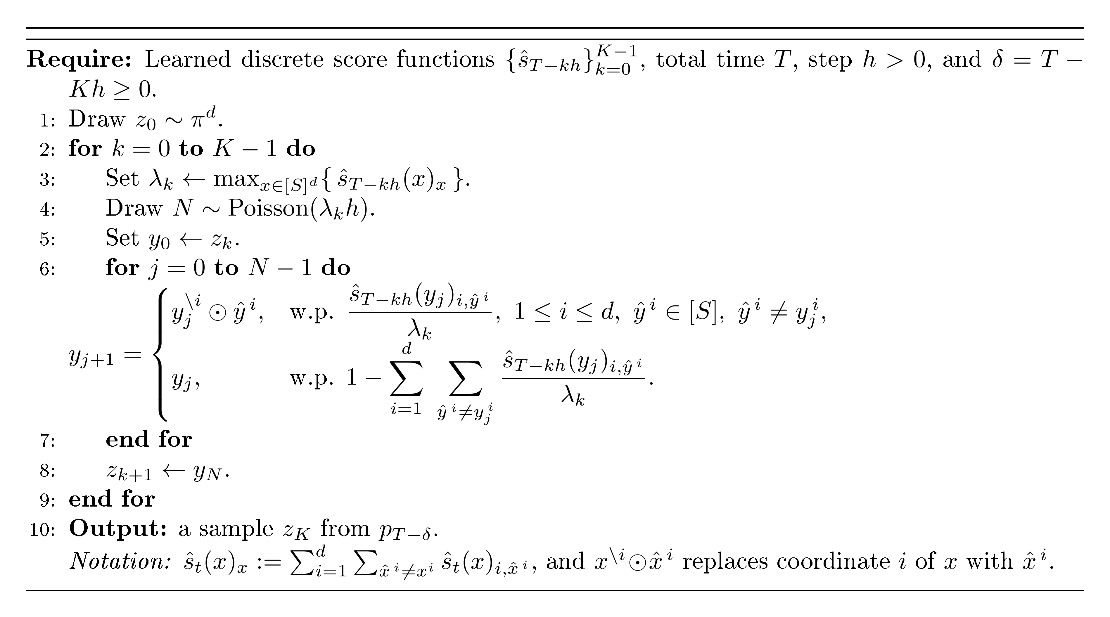
In this section, we provide a practical training and sampling algorithm for discrete-state diffusion models. The forward process (Step 6 in Algorithm 1) is based on Proposition 1 of [18] and the training happens through minimizing the empirical score entropy loss Equation (9). Algorithm 2 is from [18].
**Require:** Dataset $\mathcal{D}$ of samples $x_0 \in [S]^d$ (alphabet size $S$); diffusion time $T$; step-size $h$; early-stop $\delta \ge 0$; number of steps $K$ with $T = Kh + \delta$; network $s_\theta(x,t) \in \mathbb{R}^{d \times (S-1)}$; learning rate $\eta$; batch size $B$; epochs $E$.
1: **Per-token forward kernel:** $P_{0,t}= \tfrac{1}{S}(1-e^{-t})\, \mathbf{1} \mathbf{1}^\top + e^{-t}I$.
2: **for** epoch $=1$ **to** $E$ **do**
3:   **for** $k=0$ **to** $K-1$ **do**
4:     Sample minibatch $\{x_0^i\}_{i=1}^B \sim \mathcal{D}$.
5:     Sample $t \sim \mathrm{Unif}\!\big([kh+\delta,\,(k+1)h+\delta]\big)$.
6:     **Forward corruption (factorized CTMC):** for each sample $i$ and coord $j$,
       $x_t^{i,j} \sim \mathrm{Categorical}\!\big(P_{0,t}[\,x_0^{i,j},:\,]\big)$.
7:     **Build ratio targets:** for each $(i,j)$ and each $a \in [S],\, a \neq x_t^{i,j}$,
       $r_t^{i}(j,a)=\dfrac{P_{0,t}[x_0^{i,j},a]}{P_{0,t}[x_0^{i,j},x_t^{i,j}]}\,$.
8:     **Query score network frozen at the upper-limit of each interval:** $t'=(k+1)h+\delta$; compute $\hat{s}^i = s_\theta(x_t^i,\, t')$.
9:     **Score Entropy Loss:**
         $\displaystyle L(\theta)=\frac{1}{B}\sum_{i=1}^B \frac{1}{S} \sum_{j=1}^d \sum_{\substack{a=1\\ a\neq x_t^{i,j}}}^{S} \Big(-\,r_t^{i}(j,a)\log \hat{s}^i(j,a) + \hat{s}^i(j,a)\Big).$
10:    **Update:** $\theta \leftarrow \theta - \eta\,\nabla_\theta L(\theta)$.
11:  **end for**
12: **end for**
Discussion on $C$ Since we have access to uniform bounds for the true score functions from [@thm:lemma_score_uniform_bound], which depend on $B$, we can apply score clipping during training to ensure that the learned score functions are reliable. Specifically, we enforce the following conditions:
$ \max_{\mathbf{x} \in \mathcal{X}, , k \in {0, \ldots, K-1}} \left| \hat{s}{(k+1)h}(\mathbf{x}) \right|{\infty} \le \frac{3}{2}B. $
As a result, we can choose that
$ C = \frac{3}{2}B $
B. Supplmentary Lemmas
Definition (Bregman divergence). Let $\phi$ be a strictly convex function defined on a convex set $\mathcal{S} \subset \mathbb{R}^d$ ($d \in \mathbb{N}+$) and $\phi$ is differentiable. The Bregman divergence $D\phi(x|y) : \mathcal{S} \times \mathcal{S} \to \mathbb{R}_+$ is defined as
$ D_\phi(x|y) = \phi(x) - \phi(y) - \nabla \phi(y)^\top (x - y). $
In particular, the generalized I-divergence
$ D_I(x|y) = \sum_{i=1}^d \left[-x^i + y^i + x^i \log \frac{x^i}{y^i} \right] $
is generated by the negative entropy function $I(x) = \sum_{i=1}^d x^i \log x^i$.
The Bregman divergence does not satisfy the triangle inequality. However, when the domain of the negative entropy is restricted to a closed box contained in $\mathbb{R}_+^d$, we have the following Lemma from Proposition 3 of [18], which provides an analogous form of the triangle inequality.
########## {caption="Lemma 8"}
Let the negative entropy function $ I(x) = \sum_{i=1}^d x^i \log x^i $ be defined on $ [a, b]^d \subset \mathbb{R}_{+}^d $ for constants $ 0 < a < b $ . Then for all $ x, y, z \in [a, b]^d $, we have:
1.
$ D_I(x | y) ;\leq; \frac{1}{a}, |x - z|_2^2 ;+; \frac{2b}{a}, D_I(z | y). $
2.
$ D_I(x | y) ;\leq; \frac{1}{a}, |x-z|_2^2 ;+; \frac{b}{a^2}, |z-y|_2^2 $
Proof: Let $ I(x) = \sum_{i=1}^d x^i \log x^i $, and note that its Hessian is given by
$ \nabla^2 I(x) = \text{diag}\left(\frac{1}{x^1}, \ldots, \frac{1}{x^d} \right). $
Since $ x \in [a, b]^d $, we have
$ \frac{1}{b} I_d \preceq \nabla^2 I(x) \preceq \frac{1}{a} I_d. $
This implies that $ I $ is $ \frac{1}{b} $ -strongly convex and its gradient $ \nabla I $ is $ \frac{1}{a} $ -Lipschitz smooth.
By the second-order Taylor expansion of the Bregman divergence, there exists $ \theta \in [0, 1] $ such that
$ D_I(x | y) = \frac{1}{2} (x - y)^\top \nabla^2 I(y + \theta(x - y)) (x - y). $
Using $ \nabla^2 I(x) \preceq \frac{1}{a} I_d $, we obtain
$ D_I(x | y) \leq \frac{1}{2a} |x - y|_2^2.\tag{24} $
Now apply the triangle inequality to the right-hand side of (24):
$ |x - y|_2^2 \leq 2|x - z|_2^2 + 2|z - y|_2^2. $
Substituting into the previous inequality (24) gives
$ D_I(x | y) \leq \frac{1}{a} |x - z|_2^2 + \frac{1}{a} |z - y|_2^2.\tag{25} $
Since $ I $ is $ \frac{1}{b} $ -strongly convex, we have
$ D_I(z | y) \geq \frac{1}{2b} |z - y|_2^2 \quad \Rightarrow \quad |z - y|_2^2 \leq 2b \cdot D_I(z | y). $
Substituting this into (25) yields
$ D_I(x | y) \leq \frac{1}{a} |x - z|_2^2 + \frac{2b}{a} \cdot D_I(z | y). $
This completes the proof of the first part ((i)) of the Lemma.
Because $\nabla^2 I(x) = \mathrm{diag}(1/x^1, \ldots, 1/x^d) \preceq \tfrac{1}{a} I_d$ on $[a, b]^d$, the function $I$ is $\tfrac{1}{a}$-smooth. Hence, for $z, y$,
$ D_I(z | y) ;\leq; \frac{1}{2a}, |z-y|_2^2.\tag{26} $
Substituting this in ((i)), we obtain the following:
$ \begin{align} D_I(x | y) &;\leq; \frac{1}{a}, |x-z|_2^2 ;+; \frac{2b}{a}, D_I(z | y) \nonumber \ &;\leq; \frac{1}{a}, |x-z|_2^2 ;+; \frac{2b}{a}\cdot \frac{1}{2a}, |z-y|_2^2 \nonumber \ &;\leq; \frac{1}{a}, |x-z|_2^2 ;+; \frac{b}{a^2}, |z-y|_2^2. \end{align}\tag{27} $
It is generally a common practice to use the bounds $[1/C, C]$ instead of $[a, b]$ from Proposition 3 in [18]. By substituting $a = 1/C$ and $b = C$ in Equation (27), we obtain the following bound:
$ D_I(x , |, y) ;\le; C , |x - z|_2^2 ;+; C^3 , |z - y|_2^2. $
This proves the second part ((ii)) of the Lemma.
This completes the proof of [@thm:lemma_bregman_decomposition]
########## {caption="Lemma 9"}
The KL divergence between the true and approximate path measures of the reverse process, both starting from $q_T$, is ([18])
$ D_{\mathrm{KL}}(\mathbb{Q}, |, \mathbb{P}^{q_T}) = \sum_{k=0}^{K-1} \int_{kh+\delta}^{(k+1)h+\delta} \mathbb{E}{\mathbf{x}t \sim q_t} \sum{i=1}^d \sum{\hat{x}^i_t \neq x^i_t} Q_t^{\mathrm{tok}}(\hat{x}^i_t, x^i_t) , D_I!\left(s_t(\mathbf{x}t){i, \hat{x}^i_t} , |, \hat{s}_{(k+1)h+\delta}(\mathbf{x}t){i, \hat{x}^i_t} \right) dt. $
########## {caption="Lemma 10: Score bound - follows from Lemma 4 of [18]"}
Suppose Assumption 3 holds. Then for all $t \in [0, T]$, $\mathbf{x} \in \mathcal{X}$, $i \in [d]$ and $\hat{x}^i \neq x^i \in [S]$, we have
$ \dfrac{1}{B};\leq; s_t(\mathbf{x})_{i, \hat{x}^i} ;\leq; B. $
Proof: The Proof of [@thm:lemma_score_uniform_bound] follows from the Proof of Lemma 4 of [18] Define the kernel function
$ g_{\mathbf{w}}(t) = \frac{1}{S^{d}} \prod_{i=1}^{d} \Bigl[, 1 + e^{-t}\bigl(-1 + S\cdot \mathbf{1}{w^{i}\equiv 0 \ (\mathrm{mod}\ S)}\bigr)\Bigr], \qquad \mathbf{w}\in \mathbb{Z}^{d}, \ t\ge 0 . $
From Proposition 1 of [18], the transition probability of the forward process can be written as
$ \begin{align*} q_{t|s}(\mathbf{x}{t}\mid \mathbf{x}{s}) &= \prod_{i=1}^{d} q^{i}{t|s}(x^{i}{t}\mid x^{i}{s}) = \prod{i=1}^{d} P^{0}{s, t}(x^{i}{s}, x^{i}{t})\ &= \frac{1}{S^{d}} \prod{i=1}^{d} \Bigl[, 1 + e^{-(t-s)}\bigl(-1 + S\cdot \delta{x^{i}{t}, x^{i}{s}}\bigr)\Bigr], \qquad \forall, t>s\ge 0 . \end{align*} $
Hence $q_{t|0}(\mathbf{y}\mid \mathbf{x}) = g_{\mathbf{y}-\mathbf{x}}(t)$ for $t>0$ . Thus, for all $t\in (0, T]$, $\mathbf{x}\in \mathcal{X}$, $i\in [d]$, and $x^{i}\neq \hat{x}^{i}\in [S]$,
$ \begin{align*} s_{t}(\mathbf{x}){i, \hat{x}^{i}} &= \frac{q{t}(\mathbf{x}^{\backslash i}\odot \hat{x}^{i})}{q_{t}(\mathbf{x})} = \frac{q_{t}\bigl(\mathbf{x}+(\hat{x}^{i}-x^{i})\mathbf{e}{i}\bigr)}{q{t}(\mathbf{x})}\ &= \frac{\sum_{\mathbf{y}\in \mathcal{X}} q_{0}(\mathbf{y}), q_{t|0}\bigl(\mathbf{x}+(\hat{x}^{i}-x^{i})\mathbf{e}{i}\mid \mathbf{y}\bigr)}{q{t}(\mathbf{x})} = \frac{\sum_{\mathbf{y}\in \mathcal{X}} q_{0}(\mathbf{y}), g_{\mathbf{x}+(\hat{x}^{i}-x^{i})\mathbf{e}{i}-\mathbf{y}}(t)}{q{t}(\mathbf{x})}\ &= \frac{\sum_{\mathbf{y}\in \mathcal{X}} q_{0}\bigl(\mathbf{y}+(\hat{x}^{i}-x^{i})\mathbf{e}{i}\bigr), g{\mathbf{x}-\mathbf{y}}(t)}{q_{t}(\mathbf{x})} = \sum_{\mathbf{y}\in \mathcal{X}} \frac{q_{0}(\mathbf{y}), q_{t|0}(\mathbf{x}\mid \mathbf{y})}{q_{t}(\mathbf{x})}, \frac{q_{0}\bigl(\mathbf{y}+(\hat{x}^{i}-x^{i})\mathbf{e}{i}\bigr)}{q{0}(\mathbf{y})}\ &= \dfrac{1}{B} ;\le; \mathbb{E}{\mathbf{y}\sim q{0|t}(\cdot\mid \mathbf{x})} \Biggl[\frac{q_{0}\bigl(\mathbf{y}+(\hat{x}^{i}-x^{i})\mathbf{e}{i}\bigr)}{q{0}(\mathbf{y})}\Biggr] ;\le; B, \end{align*} $
where the last inequality uses Assumption 3. The sum $\mathbf{y}+(\hat{x}^{i}-x^{i})\mathbf{e}_{i}$ is interpreted in modulo- $S$ sense. $\square$
########## {caption="Lemma 11: Score movement bound - Lemma 5 of [18]"}
Suppose Assumption 3 holds. Let $\delta = 0$. Then for all $k \in {0, 1, \dots, K-1}$, $t \in [kh, (k+1)h]$, $\mathbf{x} \in \mathcal{X}$, $i \in [d]$, and $\hat{x}^i \neq x^i \in [S]$, we have
$ \bigl| s_t(\mathbf{x}){i, \hat{x}^i} - s{(k+1)h}(\mathbf{x})_{i, \hat{x}^i} \bigr| ;\lesssim; \left[\frac{1}{1 - e^{-(k+1)h}} + S \right] \kappa_i h. $
########## {caption="Lemma 12: Theorem 26.5 of [38]"}
Assume that for all $z$ and $h \in \mathcal{H}$ we have that $|\ell(h, z)| \leq c$.
Then,
- With probability of at least $1 - \delta$, for all $h \in \mathcal{H}$,
$ \begin{align} L_D(h) - L_S(h) \leq 2 \underset{S' \sim D^m}{\mathbb{E}} R(\ell \circ \mathcal{H} \circ S') + c\sqrt{\frac{2 \ln(2/\delta)}{m}}. \end{align} $
In particular, this holds for $h = \text{ERM}_{\mathcal{H}}(S)$. 2. With probability of at least $1 - \delta$, for all $h \in \mathcal{H}$,
$ \begin{align} L_D(h) - L_S(h) \leq 2R(\ell \circ \mathcal{H} \circ S) + 4c\sqrt{\frac{2 \ln(4/\delta)}{m}}. \end{align} $
In particular, this holds for $h = \text{ERM}_{\mathcal{H}}(S)$. 3. For any $h^*$, with probability of at least $1 - \delta$,
$ \begin{align} L_D(\text{ERM}_{\mathcal{H}}(S)) - L_D(h^*) \leq 2R(\ell \circ \mathcal{H} \circ S) + 5c\sqrt{\frac{2 \ln(8/\delta)}{m}}. \end{align} $
########## {caption="Lemma 13: Extension of Massart's Lemma"}
Let $\Theta^{''}$ be a finite function class. Then, for any $\theta \in \Theta^{''}$, we have
$ \begin{align} \mathbb{E}{\sigma} \left[\max{\theta \in \Theta^{''}}\sum_{i=1}^{n}f(\theta){\sigma_{i}} \right] \le ||f(\theta)||_{2} \le (BW)^L!\left(d+\frac{L}{W}\right) \end{align} $
where $\sigma_{i}$ are i.i.d random variables such that $\mathbb{P}(\sigma_{i} = 1) = \mathbb{P}(\sigma_{i} = -1) =\frac{1}{2}$.
We get the second inequality by denoting $L$ as the number of layers in the neural network, $W$ and $B$ a constant such all parameters of the neural network upper bounded by $B$. $d$ is the dimension of the function $f(\theta)$.
Proof: Let $h_0=x$, and for $\ell=0, \dots, L-1$ define the layer recursion
$ h_{\ell+1}=\sigma(W_\ell h_\ell + b_\ell), $
where $W_\ell\in\mathbb{R}^{n_{\ell+1}\times n_\ell}$, $b_\ell\in\mathbb{R}^{n_{\ell+1}}$, and $n_\ell\le W$ for hidden layers. We work with the $\ell_\infty$ operator norm:
$ |W_\ell|\infty=\max_i \sum_j |(W\ell){ij}| ;\le; B, n\ell ;\le; BW=\alpha. $
Since $\sigma$ is $1$ -Lipschitz with $\sigma(0)=0$, we have $|\sigma(u)|\infty\le|u|\infty$ and thus
$ |h_{\ell+1}|\infty ;\le; |W\ell|\infty, |h\ell|\infty + |b\ell|\infty ;\le; \alpha, |h\ell|_\infty + B. $
With $|h_0|_\infty\le d$, iterating this affine recursion yields the standard geometric-series bound
$ |h_L|\infty ;\le; \alpha^L d ;+; B\sum{i=0}^{L-1}\alpha^{, i} ;=; \alpha^L d ;+; B, \frac{\alpha^{L}-1}{\alpha-1} \quad(\alpha\neq 1), $
and for $\alpha=1$, $|h_L|\infty\le d+BL$ . The scalar output $f(x)$ is either a coordinate of $h_L$ or obtained by applying the same $1$ -Lipschitz activation to a linear form of $h_L$ ; in either case, $|f(x)|\le|h_L|\infty$, giving the stated bound.
For the $\alpha\ge 1$ simplification, use $\sum_{i=0}^{L-1}\alpha^i \le L\alpha^{L-1}$ to obtain
$ |f(x)| ;\le; \alpha^L d + B L \alpha^{L-1} ;=; (BW)^L!\left(d+\frac{L}{W}\right). $
For $\alpha<1$, since $\alpha^i\le 1$, $\sum_{i=0}^{L-1}\alpha^i\le L$ and hence $|f(x)|\le d+BL$ . Note that this is a tighter bound that the one for $\alpha \ge 1$. However, we retain the bound for $\alpha \ge 1$ to make our result hold for both cases.
########## {caption="Lemma 14: Theorem 4.6 of [39]"}
Let $f$ be $L$-smooth. Assume $f \in PL(\mu)$ and $g \in ER(\rho)$. Let $\gamma_k = \gamma \leq \frac{1}{1+2\rho/\mu} \cdot \frac{1}{L}$, for all $k$, then SGD update given by $x^{k+1} = x^k - \gamma^k g(x^k)$ converges as follows
$ \begin{align} \mathbb{E}[f(x^k) - f^*] \leq (1 - \gamma\mu)^k [f(x^0) - f^*] + \frac{L\gamma\sigma^2}{\mu}. \end{align} $
Hence, given $\varepsilon > 0$ and using the step size $\gamma = \frac{1}{L} \min \left{ \frac{\mu\varepsilon}{2\sigma^2}, \frac{1}{1+2\rho/\mu} \right}$ we have that
$ \begin{align} k \geq \frac{L}{\mu} \max \left{ \frac{2\sigma^2}{\mu\varepsilon}, 1 + \frac{2\rho}{\mu} \right} \log \left(\frac{2(f(x^0) - f^*)}{\varepsilon} \right) \quad \Longrightarrow \quad \mathbb{E}[f(x^k) - f^*] \leq \varepsilon. \end{align} $
########## {caption="Lemma 15: Discrete–continuous score-error: absolute $O(h)$ gap"}
Let $(X_t){t\in[\delta, T]}$ be a continuous-time Markov chain on a finite state space $\Omega$ with generator $Q=(q(x, y)){x, y\in\Omega}$, and write $q_t$ for the law of $X_t$.
Fix a stepsize $h>0$ and the grid $t_k:=\delta+kh$ for $k=0, \dots, K-1$ with intervals $I_k=[t_k, t_{k+1}]$ and $Kh=T-\delta$.
For each $k$, define
$ f_k(x);:=;D!\left(s_{t_k}(x), \big|, \hat s_{t_k}(x)\right), $
and assume a finite uniform departure rate
$ \lambda ;:=; \sup_{x\in\Omega}\sum_{y\neq x} q(x, y) ;<;\infty.\tag{28} $
Let $S\ge 1$ denote the (harmless) scaling constant.
Define the continuous- and discrete-time score-error terms
$ \mathrm{CT}:=\frac1S\sum_{k=0}^{K-1}\int_{I_k}\mathbb{E}{q_t}!\big[f_k(X)\big], dt, \qquad \mathrm{DT}:=\frac1S\sum{k=0}^{K-1} h, \mathbb{E}{q{t_k}}!\big[f_k(X)\big]. $
Then the absolute difference satisfies
$ \big|\mathrm{CT}-\mathrm{DT}\big| ;\le; \frac{(S-1){\cdot}d{\cdot}C, \lambda, T, h}{S}.\tag{29} $
Proof: Fix $k$ and set $g_k(t):=\mathbb{E}_{q_t}[f_k(X)]$ for $t\in I_k$. By the Kolmogorov forward equation $(\dot q_t = Q^\top q_t)$,
$ \frac{d}{dt}, g_k(t) =\sum_x (Q^\top q_t)(x)f_k(x) =\sum_x q_t(x), (Qf_k)(x) =\mathbb{E}_{q_t}!\big[(Qf_k)(X)\big], $
where $(Qf_k)(x)=\sum_{y\neq x} q(x, y)\big(f_k(y)-f_k(x)\big)$. Using ([@thm:lemma_score_uniform_bound]) and the triangle inequality,
$ \big|(Qf_k)(x)\big| ;\le; \sum_{y\neq x} q(x, y), \big|f_k(y)-f_k(x)\big| ;\le; \sum_{y\neq x} q(x, y)\cdot 2(S-1) dC;\le; 2(S-1)dC\lambda. $
Hence $\sup_{t\in I_k}\big|g_k'(t)\big|\le 2(S-1)dC\lambda$. From, Lemma 16 we have
$ \left|\int_{t_k}^{t_{k+1}} g_k(t), dt - h, g_k(t_k)\right| ;\le; \frac{h^2}{2}, \sup_{u\in I_k}\big|g_k'(u)\big| ;\le; 2(S-1)dC\lambda h^2 $
Summing over $k=0, \dots, K-1$ gives
$ \left|\sum_{k=0}^{K-1}\int_{I_k}!\mathbb{E}{q_t}[f_k], dt -\sum{k=0}^{K-1} h, \mathbb{E}{q{t_k}}[f_k]\right| ;\le; \sum_{k=0}^{K-1} (S-1)dC\lambda h^2 ;=; (S-1)dC\lambda Kh^2 ;\le; (S-1)dC\lambda T h, $
since $Kh=T-\delta\le T$. Dividing both sides by $S$ yields Equation (29).
If $|s_t|\infty, |\hat s_t|\infty\le C$ on $[\delta, T]$ and $D$ is a Bregman divergence whose generator is smooth on the corresponding bounded set, then $M\le c, C^2$ for a constant $c$. For single–coordinate refresh dynamics in $d$ dimensions with uniform symbol choice, $\lambda\le d, (S-1)/S$. Consequently, Equation (29) gives $\big|\mathrm{CT}-\mathrm{DT}\big|\le (c, C_1^2), d, T, h/S$.
########## {caption="Lemma 16: First-order quadrature remainder (left rectangle rule)"}
Let $g:[a, b]\to\mathbb{R}$ be absolutely continuous with $g'\in L^\infty([a, b])$.
Then
$ \int_a^b g(t), dt ;-; (b-a), g(a) ;=; \int_a^b (b-u), g'(u), du,\tag{30} $
and consequently
$ \Bigl|\int_a^b g(t), dt ;-; (b-a), g(a)\Bigr| ;\le; \frac{(b-a)^2}{2}, |g'|_{\infty, [a, b]}.\tag{31} $
Moreover, the constant $1/2$ is sharp (equality holds for affine $g(t)=\alpha+\beta t$).
Proof: By absolute continuity and the fundamental theorem of calculus, $g(t)=g(a)+\int_a^t g'(u), du$ for all $t\in[a, b]$. Integrating both sides in $t$ gives
$ \int_a^b g(t), dt = (b-a), g(a) + \int_a^b !\left(\int_a^t g'(u), du\right)!dt. $
By Tonelli/Fubini (justified since $g'\in L^\infty$),
$ \int_a^b !\left(\int_a^t g'(u), du\right)!dt = \int_a^b !\left(\int_u^b dt\right) g'(u), du = \int_a^b (b-u), g'(u), du, $
which proves Equation (30). Taking absolute values and using $0\le b-u\le b-a$,
$ \Bigl|\int_a^b (b-u), g'(u), du\Bigr| \le |g'|{\infty, [a, b]} \int_a^b (b-u), du = |g'|{\infty, [a, b]} , \frac{(b-a)^2}{2}, $
which is Equation (31). Sharpness follows by direct calculation for $g(t)=\alpha+\beta t$, where the error equals $\beta(b-a)^2/2$.
[Right rectangle, midpoint, and nonuniform steps] (1) Right rectangle. An identical argument with $g(b)$ in place of $g(a)$ yields
$ \int_a^b g(t), dt - (b-a), g(b) = -\int_a^b (u-a), g'(u), du, \qquad \Bigl|\int_a^b g(t), dt - (b-a), g(b)\Bigr| \le \frac{(b-a)^2}{2}, |g'|_\infty . $
(2) Midpoint rule (needs a second derivative). If $g'$ is absolutely continuous and $g''\in L^\infty([a, b])$, then
$ \Bigl|\int_a^b g(t), dt - (b-a), g!\left(\tfrac{a+b}{2}\right)\Bigr| \le \frac{(b-a)^3}{24}, |g''|_\infty. $
We do not use this in the theorem since we only assume a bound on $g'$.
(3) Nonuniform mesh. For intervals $I_k=[t_k, t_{k+1}]$ with $h_k=t_{k+1}-t_k$ and $g_k$ absolutely continuous on $I_k$,
$ \left|\int_{I_k} g_k(t), dt - h_k, g_k(t_k)\right| \le \frac{h_k^2}{2}, |g_k'|{\infty, I_k}, \qquad \sum_k \left|\int{I_k} g_k - h_k g_k(t_k)\right| \le \frac{1}{2}\sum_k h_k^2 |g_k'|_{\infty, I_k}. $
If $h_{\max}:=\max_k h_k$, this implies $\sum_k \left|\int_{I_k} g_k - h_k g_k(t_k)\right| \le \tfrac{h_{\max}}{2}\sum_k h_k |g_k'|_{\infty, I_k}$.
How this plugs into the theorem.
In the proof of Lemma 15, set $a=t_k$, $b=t_{k+1}$ and $g_k(t):=\mathbb{E}{q_t}[f_k(X)]$. From the CTMC calculus we had $g_k'(t)=\mathbb{E}{q_t}[(Qf_k)(X)]$ and $|g_k'|_{\infty, I_k}\le 2(S-1)dC\lambda$. Applying Lemma 16 gives the per-interval bound
$ \left|\int_{t_k}^{t_{k+1}} g_k(t), dt - h, g_k(t_k)\right| \le \frac{h^2}{2}\cdot 2(S-1)dC\lambda = M\lambda h^2. $
Summing over $k$ and using $Kh=T-\delta\le T$ yields $\big|\mathrm{CT}-\mathrm{DT}\big| \le (2(S-1)dC\lambda/S), Kh^2 \le (2(S-1)dC\lambda/S), T h$, which is exactly the absolute $O(h)$ gap.
C. Intermediate Lemmas
In this section, we present the proofs of intermediate lemmas used to bound the approximation error, statistical error, and optimization error in our analysis.
C.1 Bounding the Approximation error
Recall Lemma 5 (Approximation Error.) *Let $W$ and $D$ denote the width and depth of the neural network architecture, respectively, and let $Sd$ represent the input data dimension. Then, for all $k \in [{0}, K-1]$ we have
$ \mathcal{E}^{\mathrm{approx}}_k = 0 $
Proof: We construct a network explicitly such that it matches any given function defined on a fixed set of points. The proof has two parts: a base construction of depth $2$ (one hidden layer) and an inductive padding by identity layers that preserves the values on $X$ while increasing depth without increasing width.
We give a constructive proof. The idea is (i) build a depth-2 interpolant using only $S$ of the $W$ hidden units and zero out the remaining $W-S$, then (ii) increase depth by inserting identity blocks that act as the identity on the finite set of hidden codes, still using width $W$.
Step 0 (Distinct scalar coordinates). Since $x_1, \dots, x_S$ are distinct, choose $a\in\mathbb{R}^d$ so that $t_i:=a^\top x_i$ are pairwise distinct. Relabel so $t_1<t_2<\cdots<t_S$.
Step 1 (Depth-2 interpolant of width $W\ge S$). Pick biases $b_1, \dots, b_S$ such that
$ b_1<t_1, \qquad b_k\in\Big(\tfrac{t_{k-1}+t_k}{2}, , t_k\Big)\ \text{ for }k=2, \dots, S. $
For $\alpha>0$ define the $S\times S$ matrix $A^{(\alpha)}$ with entries
$ A^{(\alpha)}_{ik}:=\phi!\big(\alpha(t_i-b_k)\big), \qquad 1\le i, k\le S. $
As in the triangular-limit argument, the rescaled matrix
$ \widetilde A^{(\alpha)}:=\frac{A^{(\alpha)}-\phi_- \mathbf{1}\mathbf{1}^\top}{\phi_+-\phi_-} $
converges entrywise to the unit lower-triangular matrix $L$ as $\alpha\to\infty$, hence is invertible for some finite $\alpha^\star>0$. Let $y=(f(x_1), \dots, f(x_S))^\top$ and choose any $c_0\in\mathbb{R}$. Solve for $c=(c_1, \dots, c_S)^\top$ in
$ A^{(\alpha^\star)}c = y - c_0\mathbf{1}. $
Now define a one-hidden-layer network with width $W$ by using the first $S$ hidden units exactly as above and setting the remaining $W-S$ hidden units to arbitrary parameters but with output weights equal to zero. Concretely,
$ N_2(x) := c_0 + \sum_{k=1}^{S} c_k, \phi!\big(\alpha^\star(a^\top x - b_k)\big)
- \sum_{k=S+1}^{W} 0\cdot \phi(, \cdot, ). $
Then $N_2(x_i)=f(x_i)$ for all $i$. Thus we have a depth-2 interpolant of width $W$.
Step 2 (Identity-on-a-finite-set block with width $W\ge S$). We show that for any finite set $U={u_1, \dots, u_S}\subset\mathbb{R}^m$ there exists a one-hidden-layer map
$ G(u)=C, \phi!\big(\alpha(Bu+d)\big)+e, \qquad \text{(hidden width }W\ge S), $
such that $G(u_i)=u_i$ for all $i$.
Construction. Choose $S$ rows of $B$ and corresponding entries of $d$ so that the $S\times S$ matrix
$ M^{(\alpha)}_{ik}:=\phi!\big(\alpha(b_k^\top u_i + d_k)\big), \qquad 1\le i, k\le S, $
has the same lower-triangular limit as in Step 1; hence $M^{(\alpha^\star)}$ is invertible for some finite $\alpha^\star$. Let $U:=[u_1, \cdots, u_S]\in\mathbb{R}^{m\times S}$ and define $C\in\mathbb{R}^{m\times W}$ by
$ C=\big[, U, (M^{(\alpha^\star)})^{-1}\ \ \ \ 0_{m\times (W-S)}, \big], $
i.e., the last $W-S$ columns are zeros. Set the last $W-S$ rows of $B$ and entries of $d$ arbitrarily, and take $e=0$. Then for each $i$,
$ G(u_i)=C, \phi!\big(\alpha^\star(Bu_i+d)\big) = U, (M^{(\alpha^\star)})^{-1}, M^{(\alpha^\star)}_{\cdot i} = u_i. $
Hence $G$ acts as the identity on $U$ while using width $W\ge S$ (extra units are harmlessly zeroed out).
Step 3 (Depth lifting to any $L\ge2$ with width $W$). Let $h_i\in\mathbb{R}^{W}$ denote the hidden code of $x_i$ produced by the hidden layer of $N_2$ (the last $W-S$ coordinates may be arbitrary but are fixed). Apply Step 2 to $U={h_1, \dots, h_S}\subset\mathbb{R}^{W}$ to obtain a width- $W$ block $G$ with $G(h_i)=h_i$ for all $i$. Insert $G$ between the hidden layer and the output of $N_2$; this does not change the outputs on $X$. Repeating this insertion yields a depth- $L$ network of width $W$ that still satisfies $N(x_i)=f(x_i)$ for all $i$.
Combining the steps, for any $L\ge2$ and any $W\ge S$ there exists a depth- $L$, width- $W$ network with activation $\phi$ that interpolates $f$ exactly on $X$.
- The construction plainly subsumes the case $W=S$ by taking the last $W-S$ (i.e., zero) columns to be vacuous. 2) For vector-valued $f:X\to\mathbb{R}^m$, share the same hidden layers and use an $m$-dimensional linear readout, or solve the linear systems coordinate-wise; the width requirement remains $W\ge S$.
C.2 Bounding the Statistical Error
Next, we bound the statistical error $\mathcal{E}{\text{stat}}$. This error is due to estimating $s^*{\theta, k}(x_{k})$ from a finite number of samples rather than the full data distribution.
Recall Lemma 6 (Statistical Error.) *Let $n_k$ denote the number of samples used to estimate the score function at each diffusion step. Then, for all $k \in [0, K-1]$, with probability at least $1-\gamma$, we have
$ \mathcal{E}^{\mathrm{stat}}_k \leq \mathcal{O}\left((S-1)d\sqrt\frac{{{\log}\left(\frac{2}{\gamma}\right)}}{{n_k}}\right) $
Proof:
Let us define the population loss at time $k$ for $k \in [0, K-1]$ as follows:
$ \begin{aligned} \mathcal{L}k(\theta) &= \int{kh+\delta}^{(k+1)h+\delta}\mathbb{E}_{\mathbf{x}_k \sim q_t} \left[D_I \left(s_k(\mathbf{x}t) , |, \overline{s}{\theta, k}(\mathbf{x}_t) \right) \right] dt \end{aligned}\tag{32} $
The corresponding empirical loss is:
$ \widehat{\mathcal{L}}k(\theta) = \frac{1}{n_k} \sum{i=1}^{n_k} D_I\left(s_k(\mathbf{x}{k, t, i}) , |, \overline{s}{\theta, k}(\mathbf{x}_{k, t, i}) \right), \nonumber \quad t \sim \text{Unif}[kh, (k+1)h]\tag{33} $
Let $\theta^a_k$ and $\theta^b_k$ be the minimizers of $\mathcal{L}k(\theta)$ and $\widehat{\mathcal{L}}k(\theta)$, respectively, corresponding to score functions $s^a{\theta, k}$ and $s^b{\theta, k}$. By the definitions of minimizers, we can write
$ \begin{align} \mathcal{L}_k(\theta^b_k) - \mathcal{L}_k(\theta^a_k) &\le \mathcal{L}_k(\theta^b_k) - \mathcal{L}_k(\theta^a_k) + \widehat{\mathcal{L}}_k(\theta^a_k) - \widehat{\mathcal{L}}_k(\theta^b_k) \tag{a} \ &\le \underbrace{ \left| \mathcal{L}_k(\theta^b_k) - \widehat{\mathcal{L}}k(\theta^b_k) \right| }{\text{(I)}} + \underbrace{ \left| \mathcal{L}_k(\theta^a_k) - \widehat{\mathcal{L}}k(\theta^a_k) \right| }{\text{(II)}}. \tag{b} \end{align}\tag{34} $
Note that right hand side of Equation (34a) is less then the left hand side since we have added the quantity $ \widehat{\mathcal{L}}_k(\theta^a_k) - \widehat{\mathcal{L}}k(\theta^b_k)$ which is strictly positive since $\theta^{b}{k}$ is the minimizer of the function $\widehat{\mathcal{L}}_k(\theta)$ by definition. We then take the absolute value on both sides of Equation (34b) to get
$ \begin{align} |\mathcal{L}_k(\theta^b_k) - \mathcal{L}_k(\theta^a_k)| &\le \underbrace{ \left| \mathcal{L}_k(\theta^b_k) - \widehat{\mathcal{L}}t(\theta^b_k) \right| }{\text{(I)}} + \underbrace{ \left| \mathcal{L}_k(\theta^a_k) - \widehat{\mathcal{L}}k(\theta^a_k) \right| }{\text{(II)}}. \end{align}\tag{35} $
Note that this preserves the direction of the inequality since the left-hand side of Equation (34b) is strictly positive since $\theta^{a}_{k}$ is the minimizer of $\mathcal{L}_k(\theta)$ by definition.
We now bound terms (I) and (II) using standard generalization results. From Lemma 12, if the loss function is uniformly bounded over the parameter space $\Theta'' = {\theta^a_k, \theta^b_k}$, then with probability at least $1 - \gamma$, we have
$ \mathbb{E} \left[\left| \mathcal{L}_k(\theta) - \widehat{\mathcal{L}}_k(\theta) \right| \right] \le \widehat{R}(\theta) + \mathcal{O}\left(\sqrt{ \frac{ \log \frac{1}{\gamma} }{n_k} } \right), ; \forall ~ \theta \in \Theta'' $
where $\widehat{R}(\theta)$ denotes the empirical Rademacher complexity of the function class restricted to $\Theta''$. Since $\Theta''$ is a finite class (just two functions) and the inputs are finite, the loss function $\mathcal{L}_k(\theta)$ is bounded, thus, We have from Lemma 12
$ \mathbb{E} \left[\left| \mathcal{L}_k(\theta) - \widehat{\mathcal{L}}_k(\theta) \right| \right] \le \widehat{R}(\theta) + \mathcal{O}\left(\sqrt{ \frac{ \log \frac{1}{\gamma} }{n_k} } \right), ; \quad \forall ~\theta \in \Theta''.\tag{36} $
From Lemma 13 we have
$ \begin{align} \mathbb{E}{\sigma}\max{\theta \in \Theta^{''}}\sum_{i=1}^{n_k}f(\theta){\sigma_{i}} \le ||f(\theta)||_{2} \le (BW)^L!\left((S-1)d+\frac{L}{W}\right) \end{align} $
Now, the definition of $\hat{R}(\theta)$ is $\hat{R}(\theta)= \frac{1}{m} \mathbb{E}{\sigma}\max{\theta \in \Theta^{''}}\sum_{i=1}^{n}f(\theta){\sigma_{i}}$. Thus we get:
$ \mathbb{E} \left[\left| \mathcal{L}_k(\theta) - \widehat{\mathcal{L}}_k(\theta) \right| \right] \le \mathcal{O}\left(\frac{(W)^L\left((S-1)d+\frac{L}{W}\right)}{n_k}\right) + \mathcal{O}\left(\sqrt{ \frac{ \log \frac{1}{\gamma} }{n_k} } \right), ; \quad \forall ~\theta \in \Theta''.\tag{37} $
Here $||\Theta||$ is a value such that $||\Theta|| = \sup_{\theta \in \Theta^{''}}||\theta||_{\infty}$. Which implies that $\Theta$ is the norm of the maximum parameter value that can be attained in the finite function class $\Theta^{''}$, which yields:
$ \mathbb{E} \left[\left| \mathcal{L}_k(\theta) - \widehat{\mathcal{L}}_k(\theta) \right| \right] \le \mathcal{O} \left((W)^L\left((S-1)d+\frac{L}{W}\right) \sqrt{ \frac{ \log \frac{1}{\gamma} }{n_k} } \right), ; \quad \forall ~\theta \in \Theta'' $
Finally, using the Polyak-Łojasiewicz (PL) condition for $\mathcal{L}_k(\theta)$, from Assumption 1, we have from the quadratic growth condition of PL functions the following,
$ | \theta^a_k - \theta^b_k |^2 \le \mu \left| \mathcal{L}_k(\theta^a_k) - \mathcal{L}_k(\theta^b_k) \right|, $
Define the constant $L'$ as $L'$ = $\text{sup}{L'{k}}| s^a_{\theta, k}(x_k) - s^b_{\theta, k}(x_k)|^2 \le L'_k.| \theta^a_k - \theta^b_k |^2$. Then we have
$ \begin{align} | s^a_{\theta, k}(x_k) - s^b_{\theta, k}(x_k)|^2 &\le L'| \theta^a_k - \theta^b_k |^2 \ &\le L'\mu \left| \mathcal{L}_k(\theta^a_k) - \mathcal{L}_k(\theta^b_k) \right| \ &\le \mathcal{O} \left((W)^L\left((S-1)d+\frac{L}{W}\right) \sqrt{ \frac{\log \frac{1}{\gamma} }{n_k} } \right) \end{align} $
Taking expectation with respect to $x \sim q_{k}$ on both sides completes the proof.
C.3 Bounding the Optimization Error
The optimization error ($\mathcal{E}_{\text{opt}}$) accounts for the fact that gradient-based optimization does not necessarily find the optimal parameters due to limited steps, local minima, or suboptimal learning rates. This can be bounded as follows.
Recall Lemma 7 (Optimization Error) Let $ n_{k}$ be the number of samples used to estimate the score function at diffusion step $k$. If the learning rate $0 \le \eta \le \frac{1}{\kappa}$, then under Assumptions Assumption 1 and Assumption 2, for all $ k \in [0, K-1] $, the optimization error due to imperfect minimization of the training loss satisfies with probability at least $1-\gamma$
$ \mathcal{E}^{\mathrm{opt}}_k \leq \mathcal{O} \left((S-1)d\sqrt{\frac{ \log \left(\frac{2}{\gamma} \right)}{n_k}} \right). $
Proof: Let $\mathcal{E}_k^{\text{opt}}$ denote the optimization error incurred when performing stochastic gradient descent (SGD), with the empirical loss defined by:
$ \widehat{\mathcal{L}}k^i(\theta) = D_I\left(s_k(\mathbf{x}{k, t, i}) , |, \overline{s}{\theta, k}(\mathbf{x}{k, i}) \right) \quad t \sim \text{Unif}[kh, (k+1)h]\tag{33} $
The corresponding population loss is:
$ \begin{aligned} \mathcal{L}k(\theta) &= \int{kh+\delta}^{(k+1)h+\delta}\mathbb{E}_{\mathbf{x}_k \sim q_t} \left[D_I \left(s_k(\mathbf{x}t) , |, \overline{s}{\theta, k}(\mathbf{x}_t) \right) \right] dt \end{aligned}\tag{32} $
Thus, $\mathcal{E}_k^{\text{opt}}$ captures the error incurred during the stochastic optimization at each fixed time step $k$. We now derive upper bounds on this error.
From the smoothness of $ \mathcal{L}_k(\theta) $ through Assumption 2, we have
$ \begin{align} \mathcal{L}k(\theta{i+1}) \le \mathcal{L}{k}(\theta_i) + \langle \nabla \mathcal{L}k(\theta_i), \theta{i+1} - \theta_i \rangle + \frac{\kappa}{2} |\theta{i+1} - \theta_i|^2. \end{align} $
Taking conditional expectation given $ \theta_i $, and using the unbiased-ness of the stochastic gradient $ \nabla \widehat{\mathcal{L}}_k(\theta_i) $, we get:
$ \begin{align} \mathbb{E}[\mathcal{L}k(\theta{i+1}) \mid \theta_i] &\le \mathcal{L}_k(\theta_i)
- \alpha_t \left| \nabla \mathcal{L}_k(\theta_i) \right|^2 \nonumber \ &\quad + \frac{\kappa \alpha_t^2}{2} , \mathbb{E}\left[\left| \nabla \widehat{\mathcal{L}}_k(\theta_i) \right|^2 \mid \theta_i \right] \end{align} $
Now using the variance bound on the stochastic gradients using Assumption 2, we have
$ \begin{align} \mathbb{E}[|\nabla \widehat{\mathcal{L}}k(\theta_i)|^2 \mid \theta_i] \le |\nabla \mathcal{L}{k}(\theta_i)|^2 + \sigma^2, \end{align} $
Using this in the previous equation, we have that
$ \begin{align} \mathbb{E}[\mathcal{L}{k}(\theta{t+1}) \mid \theta_i] &\le \mathcal{L}_{k}(\theta_i)
- \eta \left| \nabla \mathcal{L}(\theta_i) \right|^2
- \frac{\kappa \eta^2}{2} \left(\left| \nabla \mathcal{L}(\theta_i) \right|^2 + \sigma^2 \right) \nonumber \ &= \mathcal{L}(\theta_i)
- \left(\eta - \frac{\kappa \eta^2}{2} \right) \left| \nabla \mathcal{L}(\theta_i) \right|^2
- \frac{\kappa \eta^2 \sigma^2}{2} \end{align} $
Now applying the PL inequality (Assumption 1), $|\nabla L(\theta_i)|^2 \ge 2\mu \left(L(\theta_i) - L^* \right)$, we substitute in the above inequality to get
$ \begin{align} \mathbb{E}[\mathcal{L}(\theta_{i+1}) \mid \theta_i] - \mathcal{L}^* &\le \left(1 - 2\mu \left(\eta - \frac{\kappa \eta^2}{2} \right)\right)\left(\mathcal{L}(\theta_i) - \mathcal{L}^*\right) + \frac{\kappa \eta^2 \sigma^2}{2}. \end{align} $
Define the contraction factor
$ \rho := 1 - 2\mu \left(\eta - \frac{\kappa \eta^2}{2} \right) $
Taking total expectation and defining $ \delta_k = \mathbb{E}[L(\theta_i) - L^*] $, we get the recursion:
$ \begin{align} \delta_{k+1} \le \rho \cdot \delta_k + \frac{\kappa \eta^2 \sigma^2}{2}. \end{align} $
When $ \eta \le \frac{1}{\kappa} $, we have
$ \begin{align} \eta - \frac{\kappa \eta^2}{2} \ge \frac{\eta}{2} \Rightarrow \rho \le 1 - \mu \eta. \end{align} $
Unrolling the recursion we have
$ \begin{align} \delta_k \le (1 - \mu \eta)^k \delta_0 + \frac{\kappa \eta^2 \sigma^2}{2} \sum_{j=0}^{t-1} (1 - \mu \eta)^j. \end{align} $
Using the geometric series bound:
$ \begin{align} \sum_{j=0}^{k-1} (1 - \mu \eta)^j \le \frac{1}{\mu \eta}, \end{align} $
we conclude that
$ \begin{align} \delta_k \le (1 - \mu \eta)^k \delta_0 + \frac{\kappa \eta \sigma^2}{2\mu}. \end{align} $
Hence, we have the convergence result
$ \begin{align} \mathbb{E}[\mathcal{L}(\theta_i) - \mathcal{L}^*] \le (1 - \mu \eta)^k \delta_0 + \frac{\kappa \eta \sigma^2}{2\mu}. \end{align} $
From theorem 4.6 of [39] states that this result implies a sample complexity of $\mathcal{O}\left(\frac{1}{n}\right)$ where $n$ is the number of steps of the SGD algorithm performed. Note that the result from [39] requires bounded gradient and smoothness assumption which are satisfied by Assumption 2.
Note that $\overline{s}{k}$ and $\overline{\theta}{k}$ denote our estimate of the score function and associated parameter obtained from the SGD. Also note that $\mathcal{L}^{*}$ is the loss function corresponding to whose minimizer is the neural network $s_{k}^{a}$ and the neural parameter $\theta_{k}^{a}$ is our estimated score parameter. Thus, applying the quadratic growth inequality.
$ \begin{align} \left| \overline{s}_k(\mathbf{x}_k) - s_k^a(\mathbf{x}k) \right|^2 &\le L \left| \overline{\theta}{k} - \theta_k^{a} \right|^2 \le \left| \mathcal{L}_k(\theta_k) - \mathcal{L}_k^* \right| \ &\le \mathcal{O}\left(\frac{1}{n} \right) \end{align} $
From Lemma 6, we have with probability $1 - \gamma$ that
$ \begin{align} \left| s_k^a(\mathbf{x}_k) - s_k^b(\mathbf{x}_k) \right|^2 &\le L \left| \theta^a_k - \theta^b_k \right|^2 \ &\le L \mu \left| \mathcal{L}_k(\theta^a_k) - \mathcal{L}_k(\theta^b_k) \right| \ &\le \mathcal{O} \left((W)^L\left((S-1)d+\frac{L}{W}\right) \sqrt{ \frac{ \log \frac{2}{\gamma} }{n_k} } \right) \end{align} $
Thus, we have with probability at least $1 - \gamma$,
$ \begin{align} \left| \overline{s}_{\theta, k}(\mathbf{x}k) - s^b{\theta, k}(\mathbf{x}k) \right|^2 &\le 2 \left| \overline{s}{\theta, k}(\mathbf{x}k) - s{\theta, k}^a(\mathbf{x}_k) \right|^2
- 2 \left| s^a_{\theta, k}(\mathbf{x}k) - s^b{\theta, k}(\mathbf{x}_k) \right|^2 \nonumber \ &\le \mathcal{O}\left(\log\left(\frac{1}{n} \right) \right)
- \mathcal{O}\left((W)^L\left((S-1)d+\frac{L}{W}\right) \sqrt{ \frac{ \log \frac{2}{\gamma} }{n_k} } \right) \nonumber \ &\le \mathcal{O} \left((W)^L\left((S-1)d+\frac{L}{W}\right) \sqrt{ \frac{ \log \frac{2}{\gamma} }{n_k} } \right) \end{align} $
Taking expectation with respect to $ \mathbf{x}_k \sim q_k $ on both sides completes the proof.
C.4 Bounding the Clipping Error
The clipping error ($\mathcal{E}{\text{clip}}$) accounts for the deviation of the unclipped score network $\overline{s}{\theta, k}(.)$ from the interval $[a, b]^{(S-1)d}$ . This can be bounded as follows.
########## {caption="Lemma 17: Clipping Error"}
Let $\mathcal{X} = [S]^d$ and for each $k \in [0, K-1]$ let the unclipped score be $;\overline{s}{\theta, k}(\cdot):\mathcal{X} \to \mathbb{R}^{d(S-1)}, $. Let the true score $s{k}(\cdot):\mathcal{X} \to [1/C, C]^{d(S-1)}$ and the clipped score $\hat{s}{\theta, k}(\cdot)$ be component-wise bounded in $[1/C, C]$. The clipped score $\hat{s}{\theta, k}(\cdot)$ can be component-wise restricted to $[1/C, C]$ as follows:
$ \hat{s}{\theta, k}(x_k){i, c} ;=; \min!\big{C, ;\max{1/C, ;\bar{s}{\theta, k}(x_k){i, c}}\big}, i\in[d], ; c\in[S]!\setminus!{x_k^i}. $
and hence, for any distribution $q_k$ on $\mathcal{X}$,
$ \mathbb{E}{x_k\sim q_k}!\bigl[|\hat{s}{\theta, k}(x_k)-\bar{s}{\theta, k}(x_k)|2^2\bigr] ;\le; \mathbb{E}{x_k\sim q_k}!\bigl[|\overline{s}{\theta, k}(x_k)-s_{k}(x_k)|_2^2\bigr].\tag{38} $
Proof: Partition the $d(S-1)$ component indices $(i, c)$ of the score vector according to the unclipped value:
$ \begin{align} \kappa_1(x_k) &= {(i, c): \bar{s}{\theta, k}(x_k){i, c} < a}, \qquad \kappa_2(x_k) = {(i, c): a \le \bar{s}_{\theta, k}(x_k)_{i, c} \le b}, \nonumber\ \kappa_3(x_k) &= {(i, c): \bar{s}_{\theta, k}(x_k)_{i, c} > b}. \end{align} $
By construction of the projection onto $[a, b]$, on $\kappa_1(x_k)$ we have $\hat{s}{\theta, k}(x_k){i, c}=a$; on $\kappa_2(x_k)$, $\hat{s}{\theta, k}(x_k){i, c}=\bar{s}{\theta, k}(x_k){i, c}$; and on $\kappa_3(x_k)$, $\hat{s}{\theta, k}(x_k){i, c}=b$. Therefore, the squared error decomposes as
$ \begin{align} |\hat{s}{\theta, k}(x_k)-\bar{s}{\theta, k}(x_k)|2^2 &= \sum{(i, c)\in\kappa_1(x_k)} \bigl(a - \bar{s}{\theta, k}(x_k){i, c}\bigr)^2
- \sum_{(i, c)\in\kappa_2(x_k)} \bigl(\hat{s}{\theta, k}(x_k){i, c} - \bar{s}{\theta, k}(x_k){i, c}\bigr)^2 \nonumber\ &\hspace{3em}
- \sum_{(i, c)\in\kappa_3(x_k)} \bigl(b - \bar{s}{\theta, k}(x_k){i, c}\bigr)^2. \end{align}\tag{39} $
In Equation (39), $\sum_{(i, c)\in\kappa_2(x_k)} \bigl(\hat{s}{\theta, k}(x_k){i, c} - \bar{s}{\theta, k}(x_k){i, c}\bigr)^2 = 0$ as $\hat{s}{\theta, k}(x_k){i, c}=\bar{s}{\theta, k}(x_k){i, c}$ on $\kappa_2(x_k)$. Since $s_{k}(x_k)_{i, c}\in[a, b]$ component-wise, the projection onto $[a, b]$ is non-expansive in each coordinate. Concretely, for $(i, c)\in\kappa_1(x_k)$,
$ \bigl(a - \bar{s}{\theta, k}(x_k){i, c}\bigr)^2 ;\le; \bigl(\bar{s}{\theta, k}(x_k){i, c} - s_{k}(x_k)_{i, c}\bigr)^2,\tag{40} $
for $(i, c)\in\kappa_3(x_k)$,
$ \bigl(b - \bar{s}{\theta, k}(x_k){i, c}\bigr)^2 ;\le; \bigl(\bar{s}{\theta, k}(x_k){i, c} - s_{k}(x_k)_{i, c}\bigr)^2,\tag{41} $
and for $(i, c)\in\kappa_2(x_k)$ we have equality
$ \bigl(\hat{s}{\theta, k}(x_k){i, c} - \bar{s}{\theta, k}(x_k){i, c}\bigr)^2 = 0.\tag{42} $
Summing Equation (40)-Equation (42) over the three index sets and using Equation (39) followed by taking expectation over $x\sim q_k$ proves Equation (38).
D. Proof of the Main Theorem
D.1 Path measure KL decomposition
The following decomposition follows from the Proof of Theorem 2 from [18].
$ \begin{align} D_{\mathrm{KL}}(\mathbb{Q}, |, \mathbb{P}^{q_T}) &= \frac{1}{S} \sum_{k=0}^{K-1} \int_{kh}^{(k+1)h} \mathbb{E}{\mathbf{x}t \sim q_t} D_I!\left(s_t(\mathbf{x}t), |, \hat{s}{(k+1)h}(\mathbf{x}t)\right) dt \nonumber \ &;\overset{(i)}{\lesssim}; \frac{C}{S} \sum{k=0}^{K-1} \int{kh}^{(k+1)h} \mathbb{E}{\mathbf{x}t \sim q_t} \bigl| s_t(\mathbf{x}t) - s{(k+1)h}(\mathbf{x}t) \bigr|2^2 , dt \nonumber \ &\quad + \frac{C^2}{S} \sum{k=0}^{K-1} \int{kh}^{(k+1)h} \mathbb{E}{\mathbf{x}t \sim q_t} D_I!\left(s{(k+1)h}(\mathbf{x}t), |, \hat{s}{(k+1)h}(\mathbf{x}t)\right) dt \nonumber \ &;\overset{(ii)}{\lesssim}; \frac{C}{S} \sum{k=0}^{K-1} \int_{kh}^{(k+1)h} \mathbb{E}{\mathbf{x}t \sim q_t} \sum{i=1}^d \sum{\hat{x}^i \neq x^i} \bigl| s_t(\mathbf{x}t){i, \hat{x}^i} - s_{(k+1)h}(\mathbf{x}t){i, \hat{x}^i} \bigr|^2 dt \nonumber \ &\quad + \frac{C^3}{S} \sum_{k=0}^{K-1} \int_{kh+\delta}^{(k+1)h+\delta} \mathbb{E}{\mathbf{x}t \sim q_t} \bigl| s{(k+1)h+\delta}(\mathbf{x}t) - \hat{s}{\theta, (k+1)h+\delta}(\mathbf{x}t) \bigr|2^2 , dt \nonumber \ &;\overset{(iii)}{\lesssim}; \frac{C}{S} \sum{k=0}^{K-1} \int{kh}^{(k+1)h} \mathbb{E}{\mathbf{x}t \sim q_t} \sum{i=1}^d \sum_{\hat{x}^i \neq x^i} \left[\frac{1}{1 - e^{-(k+1)h}} + S \right]^2 \kappa_i^2 h^2 , dt \nonumber \ &\quad + \frac{C^3}{S} \sum_{k=0}^{K-1} h , \mathbb{E}{\mathbf{x}{(k+1)h+\delta} \sim q_{(k+1)h+\delta}} \bigl| s_{(k+1)h+\delta}(\mathbf{x}_{(k+1)h+\delta})
- \hat{s}{\theta, (k+1)h+\delta}(\mathbf{x}{(k+1)h+\delta}) \bigr|_2^2
- \frac{C(S-1)d\lambda T h}{S} \nonumber \ &;\overset{(iv)}{\lesssim}; C \sum_{k=0}^{K-1} \sum_{i=1}^d \left[\frac{1}{(1-e^{-(k+1)h})^2} + S^2 \right] \kappa_i^2 h^3 \nonumber \ &\quad + \frac{C^3}{S} \sum_{k=0}^{K-1} h , A_k
- \frac{C(S-1)d\lambda T h}{S} \nonumber \ &;\overset{(v)}{\lesssim}; C \kappa^2 h^3 \int_h^T \frac{1}{(1-e^{-x})^2} dx
- C \kappa^2 S^2 h^2 T \nonumber \ &\quad + \frac{C^3}{S} \sum_{k=0}^{K-1} h , A_k
- \frac{C(S-1)d\lambda T h}{S} \nonumber \ &;\overset{(vi)}{\lesssim}; C \kappa^2 h^3 \bigl[T - \log h + \tfrac{1}{h} \bigr]
- C \kappa^2 S^2 h^2 T \nonumber \ &\quad + \frac{C^3}{S} \sum_{k=0}^{K-1} h , A_k
- \frac{C(S-1)d\lambda T h}{S} \nonumber \ &;\overset{(vii)}{\lesssim}; C \kappa^2 h^2 T (h + S^2) \nonumber \ &\quad + \frac{C^3}{S} \sum_{k=0}^{K-1} h , A_k
- \frac{C(S-1)d\lambda T h}{S} \nonumber \ &;\overset{(viii)}{\lesssim}; C \kappa^2 S^2 h^2 T \nonumber \ &\quad + \frac{C^3}{S} \sum_{k=0}^{K-1} h , A_k
- \frac{C(S-1)d\lambda T h}{S}. \end{align}\tag{43} $
The first equality follows from Lemma 9. [@thm:lemma_bregman_decomposition] $(i)$ and [@thm:lemma_score_uniform_bound] lead to the first inequality $(i)$. We particularly avoid the assumption $\frac{1}{S} \sum_{k=0}^{K-1} \int_{kh}^{(k+1)h} \mathbb{E}_{\mathbf{x}t \sim q_t}, D_I!\left(s{(k+1)h}(\mathbf{x}t), |, \hat{s}{\theta, (k+1)h}(\mathbf{x}t)\right) dt \le \varepsilon{\text{score}}$ from [18] and further upper bound it by squared L2 norm, leading to the second inequality $(ii)$. The third inequality $(iii)$ arises from [@thm:lemma_score_movement_bound_full_support] and Lemma 15. The fourth inequality $(iv)$ stems from the fact that $(a+b)^2 \leq 2(a^2+b^2)$. The sixth inequality $(vi)$ is a consequence of $e^x - 1 \geq x$, and the final inequality $(viii)$ is due to the assumption that $h \leq S^2$.
D.2 KL divergence bound
From [18] we use the result that $D_{\mathrm{KL}}(q_T , |, \pi^d) = de^{-T}\log S$. Hence, by writing $M = C(S-1)d$ the final bound on $D_{KL}(p_{data} , |, p_{T})$ from Equation (13) and (43):
$ D_{KL}(p_{data} , |, p_{T}) ;\lesssim; de^{-T}\log S + C \kappa^2 S^2 h^2 T
- \frac{C^3}{S} \sum_{k=0}^{K-1} h A_k + \frac{M\lambda T h}{S}.\tag{44} $
We shall now focus on bounding the third term in Equation (44) which expresses the score approximation error by writing $A_k = \mathbb{E}{\mathbf{x}{(k+1)h} \sim q_{(k+1)h}} \left| s_{(k+1)h}(\mathbf{x}{(k+1)h}) - \hat{s}{\theta, (k+1)h}(\mathbf{x}{(k+1)h}) \right|2^2$. For notational simplicity we re-write $A_k = \mathbb{E}{\mathbf{x}k \sim q_k} \left| s_k(\mathbf{x}k) \right. - \left. \hat{s}{\theta, k}(\mathbf{x}k) \right|2^2$ as mentioned above Equation (18). For $D{\mathrm{KL}}(q{0} | p{T}) \leq \tilde{O}(\epsilon)$ to hold, we have to ensure that each of the terms from Equation (44) scales as $\tilde{O}(\epsilon)$. Therefore, we bound the score-approximation error term $\frac{C^3}{S} \sum{k=0}^{K-1} h , \mathbb{E}{\mathbf{x}{(k+1)h} \sim q_{(k+1)h}} \bigl| s_{(k+1)h}(\mathbf{x}{(k+1)h}) - \hat{s}{\theta, (k+1)h}(\mathbf{x}_{(k+1)h}) \bigr|2^2$ based on the number of samples $n_k$ required to achieve an $\epsilon{score}$-accurate score estimator.
$ D_{KL}(q , |, p_{T}) ;\lesssim; de^{-T}\log S ;+; C \kappa^2 S^2 h^2 T ;+; \frac{C^3}{S}\sum_{k=0}^{K-1} h A_k ;+; \frac{M\lambda T h}{S} $
$ de^{-T}\log S ;\le; \epsilon \quad\Longrightarrow\quad T ;\gtrsim; \log!\Big(\tfrac{d\log S}{\epsilon}\Big)\tag{45} $
$ C \kappa^2 S^2 h^2 T ;\le; \epsilon ;;\Longrightarrow;; h ;\lesssim; \Big(\tfrac{\epsilon}{C \kappa^2 S^2 T}\Big)^{1/2}, \qquad \frac{M\lambda T h}{S} ;\le; \epsilon ;;\Longrightarrow;; h ;\lesssim; \tfrac{\epsilon S}{M\lambda T}\tag{46} $
$ h ;\lesssim; \min!\left{ \Big(\tfrac{\epsilon}{C \kappa^2 S^2 T}\Big)^{1/2}, ;\tfrac{\epsilon S}{M\lambda T} \right}\tag{47} $
$ K ;=; \frac{T}{h} ;\gtrsim; \max!\left{ T, \Big(\tfrac{C \kappa^2 S^2 T}{\epsilon}\Big)^{1/2}, ;\tfrac{M\lambda}{\epsilon}, \tfrac{T^2}{S} \right}\tag{48} $
$ T \asymp \log!\Big(\tfrac{d\log S}{\epsilon}\Big) ;\Longrightarrow; K ;\gtrsim; \max!\left{ \sqrt{\tfrac{C \kappa^2 S^2}{\epsilon}}, \big[\log(\tfrac{d\log S}{\epsilon})\big]^{3/2}, ;\tfrac{M\lambda}{\epsilon S}, \big[\log(\tfrac{d\log S}{\epsilon})\big]^2 \right}\tag{49} $
$ D_{\mathrm{KL}}(p_{\text{data}} , |, p_T) ;\le; \tilde{O}!\left(\epsilon ;+; \frac{C^{3}}{S}\sum_{k=0}^{K-1} h, A_k \right) $
Using the following bounds from earlier proofs: Bound on $\mathcal{E}_k^{\mathrm{stat}}$ from Lemma 6 and $\mathcal{E}_k^{\mathrm{opt}}$ from Lemma 7 as follows,
$\mathcal{E}_k^{\mathrm{stat}} \leq \mathcal{O} \left((W)^L\left((S-1)d+\frac{L}{W}\right) \sqrt{ \frac{\log \frac{1}{\gamma} }{n_k} } \right)$ and $\mathcal{E}_k^{\mathrm{opt}} \leq \mathcal{O} \left((W)^L\left((S-1)d +\frac{L}{W}\right) \cdot \sqrt{ \frac{ \log \frac{2}{\gamma} }{n_k} } \right)$
we obtain the following bound on $A_k$ which holds with a probability of at least $1-\gamma$:
$ \begin{align} A_k &\le \underbrace{\mathcal{O} \left((W)^L\left((S-1)d +\frac{L}{W}\right) \sqrt{ \frac{\log \frac{1}{\gamma} }{n_k} } \right) }{\text{Statistical Error}} + \underbrace{ \mathcal{O} \left((W)^L\left((S-1)d +\frac{L}{W}\right) \cdot \sqrt{ \frac{ \log \frac{2}{\gamma} }{n_k} } \right) }{\text{Optimization Error}} \ &\le \mathcal{O} \left((W)^L\left((S-1)d +\frac{L}{W}\right) \cdot \sqrt{ \frac{ \log \frac{2}{\gamma} }{n_k} } \right) \end{align}\tag{50} $
We obtain (50) by appropriately combining the statistical and optimization error terms. We have to ensure that $A_k$ satisfies the bound in (50) by setting the parameters $n_k$ (sample size at discrete time-step $k$). Simultaneously, $A_k$ must also satisfy the following inequality to ensure that the score approximation error is less than $\epsilon_{score}$, which is the desired level of accuracy that we want to achieve, and characterize it with the number of samples and the neural network parameters required. We thus shift the analysis from an assumption of access to $\epsilon_{score}$-accurate score estimator to a learning-theoretic view by characterizing the number of samples $n_k$ and network parameters $WD$ required to achieve it.
$ \frac{1}{S} \sum_{k=0}^{K-1} h , A_k \leq \epsilon_{\mathrm{score}}.\tag{51} $
where $\epsilon_{score}$ is the desired accuracy of the score estimator.
$ A_k \leq \frac{S}{Kh} , \epsilon_{\mathrm{score}}.\tag{52} $
which we obtain as the worst-case bound on the per-discrete time-step squared L2 error. Here, we specifically note that the bound on $A_k$ does not depend on $k$ since the number of samples required to train at the $k^{th}$ time-step is available across all time-steps i.e., $n_k = n$.
We isolate the two sources of error: statistical and optimization. We will solve for the sample size $ n_k = n $ .
So the bound on $A_k$ becomes:
$ A_k ;\le; \frac{S}{Kh}, \epsilon_{\text{score}} ;=; O!\left(\frac{S}{Kh, C^3}\right).\tag{53} $
To ensure the above inequality holds, we enforce:
$ W^{, L}\left((S-1)d+\frac{L}{W}\right)\sqrt{\frac{\log(2/\gamma)}{n_k}} ;\le; \frac{S}{T, C^{3}}, \epsilon.\tag{54} $
$ n_k ;\gtrsim; \frac{C^{6}, T^{2}}{S^{2}\epsilon^{2}}; W^{, 2L}!\left((S-1)d+\frac{L}{W}\right)^{2}; \log!\Big(\tfrac{2}{\gamma}\Big)\tag{55} $
In Equation (55), recall that $Kh = T$, and $T$ can be set as $T \simeq \log!\big(\tfrac{d\log S}{\epsilon}\big)$ from Equation (45).
$ n_k ;\gtrsim; \frac{C^{6}}{S^{2}\epsilon^{2}}, W^{2L}!\left(, (S-1)d+\frac{L}{W}\right)^{2} \Bigl[\log!\Bigl(\tfrac{d\log S}{\epsilon}\Bigr)\Bigr]^{2}, \log!\Bigl(\tfrac{2}{\gamma}\Bigr).\tag{56} $
Hiding the logarithmic factors, we obtain the following bound:
$ n_k ;=; \tilde{\Omega}!\left(\frac{C^{6}}{S^{2}\epsilon^{2}}; W^{, 2L}!\left((S-1)d+\frac{L}{W}\right)^{2} \right)\tag{57} $
This completes the proof of the main theorem.
E. Hardness of Learning in Discrete-State Diffusion Models
########## {caption="Lemma 18: Hardness of Learning in Discrete-State Diffusion Models"}
The generation of diffusion models with KL gap
lt;\epsilon$ needs at least $\Theta(1/\epsilon^2)$ samples for some distribution.To show this result, we will provide a construction which provides a counterexample showing that one cannot learn discrete distributions within $\varepsilon$-KL error using fewer than $\Theta(1/\varepsilon^2)$ samples. Otherwise, such a learner would violate the classical mean-estimation lower bound.
Setup. Let $x_0, x_1\in\mathbb{R}$ with $x_0\neq x_1$, and $0<\varepsilon<\tfrac{1}{25}$. Define two-point laws
$ P=(1-\varepsilon), \delta_{x_0}+\varepsilon, \delta_{x_1}, \qquad Q=(1-25, \varepsilon), \delta_{x_0}+25, \varepsilon, \delta_{x_1}.\tag{58} $
Then
$ \mathbb{E}_P[X]=x_0+\varepsilon, (x_1-x_0), \qquad \mathbb{E}_Q[X]=x_0+25, \varepsilon, (x_1-x_0), $
$ \mathrm{Var}_P(X)=\varepsilon(1-\varepsilon), (x_1-x_0)^2, \qquad \mathrm{Var}_Q(X)=(25, \varepsilon)(1-25, \varepsilon), (x_1-x_0)^2, $
so both means and variances are $\Theta(\varepsilon)$ when $|x_1-x_0|=\Theta(1)$.
For the two-point laws,
$ D_{\mathrm{KL}}(P|Q) =(1-\varepsilon)\log\frac{1-\varepsilon}{1-25\varepsilon} +\varepsilon\log\frac{\varepsilon}{25\varepsilon}. $
Using $\log(1-t)=-t-\tfrac{t^2}{2}+O(t^3)$ and $\log\frac{\varepsilon}{25\varepsilon}=\log\frac{1}{25}$, we get
$ D_{\mathrm{KL}}(P|Q) =\bigl(24-\log 25\bigr)\varepsilon + O(\varepsilon^{2}) =, c_1, \varepsilon+O(\varepsilon^{2}), $
with $c_1\approx 20.78$. As $\varepsilon\to0$, the leading term dominates, and hence $D_{\mathrm{KL}}(P|Q)=\Theta(\varepsilon)$.
Hellinger-based KL separation. For two-point laws supported on ${x_0, x_1}$ with masses $(1-p, p)$ and $(1-q, q)$, the squared Hellinger distance is
$ H^2\big((1-p, p), (1-q, q)\big)=1-\Big(\sqrt{(1-p)(1-q)}+\sqrt{pq}\Big). $
Substituting $p=\varepsilon$ and $q=25, \varepsilon$ gives
$ H^2(P, Q)=1-\sqrt{(1-\varepsilon)(1-25, \varepsilon)}-\sqrt{25}, \varepsilon. $
Using $\sqrt{1-t}\le 1-\tfrac{t}{2}$ for $t\in[0, 1]$ with $t=26\varepsilon-25\varepsilon^2$, we have
$ \sqrt{(1-\varepsilon)(1-25, \varepsilon)}\le 1-13, \varepsilon+12.5, \varepsilon^2, $
and hence
$ H^2(P, Q)\ge (13-5)\varepsilon-12.5, \varepsilon^2 =8, \varepsilon-12.5, \varepsilon^2>7.5, \varepsilon \quad\text{for all }0<\varepsilon<\tfrac{1}{25}.\tag{59} $
Implication for learners. Suppose a learner outputs a distribution $R$ such that for the unknown $U\in{P, Q}$,
$ D_{\mathrm{KL}}(U|R)\le \varepsilon. $
Since $H^2(P, Q)\le D_{\mathrm{KL}}(P|Q)$, we have $H(U, R)\le \sqrt{\varepsilon}$. Let $V$ be the other element of ${P, Q}$. By the triangle inequality for the Hellinger distance and 59,
$ H(R, V)\ge H(P, Q)-H(U, R)
\sqrt{7.5, \varepsilon}-\sqrt{\varepsilon} =(\sqrt{7.5}-1)\sqrt{\varepsilon}, $
and therefore
$ D_{\mathrm{KL}}(R|V)\ge H^2(R, V)\ge (\sqrt{7.5}-1)^2, \varepsilon>3, \varepsilon>\varepsilon. $
Thus, a learner within $\varepsilon$-KL of one distribution must be at least a constant factor more than $\varepsilon$ away from the other.
Mean-testing consequence. Setting $x_0=0$ and $x_1=1$, the mean gap is
$ \Delta=|\mathbb{E}_P[X]-\mathbb{E}_Q[X]|=24, \varepsilon, $
and the variances are bounded by constants. Assume that from $n$ samples of the true distribution, a learner can construct a simulator $R$ such that $D_{\mathrm{KL}}(U|R)\le\varepsilon$ for the true $U\in{P, Q}$. Suppose we are given $n$ samples from one of $P$ or $Q$ (unknown to us), and we use them to produce such a simulator $R$. Since $R$ is within $\varepsilon$-KL of one distribution but more than $\varepsilon$ away from the other as proved above, we can generate arbitrarily many samples from $R$ and thereby determine whether the original samples came from $P$ or from $Q$. Thus, the ability to learn a simulator $R$ within $\varepsilon$-KL error implies the ability to distinguish $P$ from $Q$.
Although $P$ and $Q$ are separated by $D_{\mathrm{KL}}(P|Q) > 20\varepsilon$, their means differ only by $\Theta(\varepsilon)$, i.e., their separation is linear in $\varepsilon$. If a simulator $R$ achieves $D_{\mathrm{KL}}(U|R) \le \varepsilon$ for some $U \in {P, Q}$, it cannot simultaneously satisfy this bound for both distributions. Therefore, distinguishing whether the samples originated from $P$ or $Q$ means that we can distinguish two distributions whose means differ by $\Theta(\varepsilon)$. By standard mean-testing lower bounds ([40]), distinguishing two distributions whose means differ by $\Theta(\varepsilon)$ requires at least $\Omega(1/\varepsilon^2)$ samples. Hence, any learner that produces such an $R$ with $D_{\mathrm{KL}}(U|R)\le\varepsilon$ must necessarily use $\Omega(1/\varepsilon^2)$ samples.
$\square$
F. Dimension of the discrete-state score
In principle, if we view the discrete-state diffusion process as a continuous-time Markov chain (CTMC) on the full state space $\mathcal{X} = [S]^d$ with $N = S^d$ states, then the forward rate matrix $Q_t$ would be of size $N \times N$, and the corresponding discrete-state score $s_t(\mathbf{x}) = \bigl(q_t(\mathbf{y})/q_t(\mathbf{x})\bigr)_{\mathbf{y} \neq \mathbf{x}}$ would indeed live in $\mathbb{R}^{N-1}$. However, such a formulation is computationally intractable for high-dimensional data.
Following prior works ([17]) and ([18]), we impose a coordinate-wise (token-wise) factorization of the forward process. Specifically, each of the $d$ coordinates evolves independently according to a shared $S \times S$ rate matrix. Under this assumption, every jump of the forward CTMC modifies exactly one coordinate at a time, and transitions are only allowed between states whose Hamming distance is one. As a result, the full rate matrix $Q_t$ is extremely sparse: from any state $\mathbf{x} \in [S]^d$, there are only $d(S-1)$ nonzero off-diagonal transitions.
The reverse-time CTMC inherits exactly the same sparsity structure. Its rate matrix $Q_t^{\leftarrow}$ involves only transitions of the form
$ \mathbf{x} ;\longrightarrow; \mathbf{x}_{\setminus i} \odot \hat{x}_i, \qquad i \in [d], \ \hat{x}_i \neq x_i, $
and for each such transition the reverse rate is given by
$ Q_t^{\leftarrow}!\left(\mathbf{x}, \mathbf{x}_{\setminus i} \odot \hat{x}i\right) ;=; Q^{\mathrm{tok}}{T-t}(\hat{x}i, x_i), \frac{q_t(\mathbf{x}{\setminus i} \odot \hat{x}_i)}{q_t(\mathbf{x})}. $
Thus, the only probability ratios that appear in the reverse dynamics are those corresponding to single-coordinate replacements.
This observation leads us to express the discrete-state score in the form required by the reverse-time CTMC. We therefore define
$ s_t(\mathbf{x})_{i, \hat{x}i} ;:=; \frac{q_t(\mathbf{x}{\setminus i} \odot \hat{x}_i)}{q_t(\mathbf{x})}, \qquad i \in [d], \ \hat{x}_i \neq x_i, $
which parametrizes all nonzero transition rates of $Q_t^{\leftarrow}$. For each coordinate $i$, the collection ${ s_t(\mathbf{x})_{i, \hat{x}_i} : \hat{x}_i \neq x_i }$ has $S-1$ degrees of freedom, since the probabilities over the $S$ possible symbols at that coordinate must sum to one after normalization. Aggregating across all $d$ coordinates yields a score representation in $\mathbb{R}^{d(S-1)}$.
Importantly, this reduction from $\mathbb{R}^{S^d-1}$ to $\mathbb{R}^{d(S-1)}$ is not an approximation or modeling choice. It is a consequence of the sparsity of the forward and reverse generators under the factorized CTMC assumption, and it provides a complete and tractable characterization of the reverse diffusion dynamics.
G. PL Condition and Sample-complexity Scaling
This section clarifies the role of the Polyak–Łojasiewicz (PL) condition in our analysis and explains how the stated sample-complexity bounds should be interpreted.
G.1 Role and Interpretation of the PL Condition
This section clarifies the role of the Polyak–Łojasiewicz (PL) condition in the analysis and explains how it should be interpreted within the theoretical framework of our work.
The PL condition is imposed as a structural regularity assumption on the population loss landscape $\mathcal{L}_k(\theta)$ at each discrete time index $k$. Its purpose is to enable control of the optimization error by relating the gradient norm to function-value suboptimality. Importantly, this assumption is not tied to strong convexity, nor is it intended to characterize the degree of overparameterization of the neural network used to parameterize the score.
While overparameterized neural networks form one prominent class of models where PL-type or gradient-dominance conditions are known to hold, such conditions have been established in substantially broader settings. In particular, PL or closely related gradient-dominance properties are known to hold even in regimes that are not heavily overparameterized, i.e., when the number of parameters doesn't exceed the number of effective constraints.
Prior work by [40] rigorously characterizes gradient-dominance and regularity conditions for several nonconvex architectures, including deep linear networks, deep linear residual networks, and one-hidden-layer nonlinear networks, in neighborhoods of global minimizers, without requiring a heavily overparameterized regime. These results show that even relatively modestly sized networks can exhibit a PL-type landscape, at least locally around solutions. This type of geometric behavior is precisely what is required in our analysis: a condition ensuring that small gradient norms imply small suboptimality, which in turn yields linear-type convergence rates for stochastic gradient methods.
In our framework, the PL condition is imposed on each time-indexed population loss $\mathcal{L}_k(\theta)$, rather than on the empirical objective. It is used solely as an analytical device to convert bounds on gradient norms into bounds on function-value suboptimality, thereby enabling control of both statistical and optimization errors. The sample-complexity requirement appearing in the main results should therefore be interpreted as a sufficient condition ensuring that these errors are controlled at the desired level. This requirement does not preclude the population loss from satisfying a PL condition in regimes where the number of samples is comparable to, or larger than, the number of trainable parameters.
G.2 Sample-Complexity Scaling and Width Assumptions
This section clarifies the interpretation of the sample-complexity bounds derived in the paper and explains the role of the width condition appearing in Lemma 5.
The main analysis yields a sample-complexity bound of the form
$ n \gtrsim \Omega!\left(W^{2L}\right), $
where $W$ denotes the width of the neural network parameterizing the score function and $L$ denotes its depth. This dependence arises from standard Rademacher complexity arguments for deep neural networks, which are known to be conservative, particularly with respect to depth. As a result, the bound should be interpreted as a worst-case sufficient condition ensuring convergence, rather than as a sharp or practically tuned estimate of the number of training samples required. Exponential or highly pessimistic depth dependence is common in current deep-learning theory such as in [41] and often substantially overestimates actual data requirements.
When this bound is combined with the sufficient-width condition $W \ge (S-1)d$ used in Lemma 1, the resulting scaling becomes $\Omega((Sd)^{2L})$, which can be numerically large for large vocabularies $S$ or deep networks $L$. This behavior reflects the proof technique and worst-case generalization guarantees rather than an inherent limitation of discrete-state diffusion models. Importantly, the substitution $W = (S-1)d$ is not required by the main generalization theorem itself; it is introduced solely as a convenient sufficient condition in Lemma 5 to ensure zero approximation error via an explicit construction.
More generally, when $W < (S-1)d$ such as with parameter sharing or low-rank structure, the analysis extends naturally by introducing an explicit approximation error term. Let
$ \varepsilon_{\mathrm{approx}}(W, S, d) $
denote the infimum over all width- $W$ networks in the considered class of the population approximation error to the target score function. Under this formulation, Lemma 5 and the main excess-risk bound can be restated with an additional additive term $\varepsilon_{\mathrm{approx}}(W, S, d)$. In the special case $W \ge (S-1)d$, the explicit construction implies $\varepsilon_{\mathrm{approx}}(W, S, d)=0$, recovering the original statement of Lemma 5.
This perspective is standard in learning theory. Approximation error induced by restricting to a given function class is often treated as a fixed constant once the class is chosen, allowing the analysis to focus on estimation and optimization errors that depend on the sample size. For example, in PAC-Bayesian analyses, approximation or misspecification errors are absorbed into a constant term once the hypothesis class is fixed ([42]). Similarly, in NTK or RKHS based analyses of neural networks, it is typically assumed that the target function lies in, or is well approximated by, the chosen function class, with the resulting misspecification error represented as a constant additive term ([43]). Existing theoretical analyses of diffusion models adopt analogous assumptions, treating approximation error as fixed ([24, 44, 37]).
H. Relationship to Prior Work
This work is inspired by existing theoretical analyses of discrete-state diffusion models ([18, 17]), particularly those that decompose the overall error into interpretable components and study convergence under idealized assumptions. Similar decomposition is used in works in reinforcement learning such as [45, 46, 48]. We adopt a similar high-level decomposition as a conceptual starting point, but develop technical tools and results tailored to discrete-state diffusion models trained with finite-width neural networks under nonconvex objectives.
At a high level, the novelty of this work lies in making the abstract components of prior discrete-state diffusion analyses explicit, data-dependent, and architecture-aware in the discrete-state setting.
Approximation error (Lemma 5).
Prior analyses typically assume realizability of the score function or work in a fixed functional class, thereby avoiding explicit treatment of approximation error. In contrast, Lemma 5 provides a discrete-state-specific approximation result that characterizes when a finite-width neural network can approximate the discrete-state score function and how this depends on the vocabulary size $S$ and dimension $d$. This lemma explicitly connects neural network expressivity to the statistical behavior of discrete-state diffusion models, a connection that does not appear in existing analyses.
Statistical error (Lemma 6).
While previous works derive convergence bounds at an abstract functional level, our analysis yields an explicit, training data dependent sample-complexity bound under a nonconvex PL-type landscape. This result makes the residual error term in prior analyses concrete and interpretable in terms of network width, depth, vocabulary size, and diffusion time. As a result, the statistical component of the error decomposition becomes an explicit quantity rather than an implicit asymptotic remainder.
Optimization error (Lemma 7).
We further analyze how optimization error propagates through the diffusion time horizon. This discrete-time stability analysis quantifies how local errors accumulate across steps and affect the final generated distribution. Such propagation effects are absent from prior analyses as they assume access to an empirical risk minimizer (ERM) and are essential for understanding convergence in the discrete-state setting with finite optimization steps.
Together, these results extend existing theory to a substantially more realistic setting, yielding guarantees that are not accessible through existing analyses.
References
Section Summary: This references section lists over 30 academic papers and books that underpin research on diffusion models, a type of AI technology for generating data like images, text, and molecules. The sources explore core concepts such as score-based generative modeling, efficient applications in vision and drug discovery, probabilistic time series, and text generation, alongside theoretical studies on convergence, optimization, and sample complexity in machine learning. Spanning from 2011 to 2026, the citations draw from major conferences like NeurIPS and ICLR, as well as journals and arXiv preprints.
[1] Song et al. (2021). Score-Based Generative Modeling through Stochastic Differential Equations. In ICLR.
[2] Ulhaq, Anwaar and Akhtar, Naveed (2022). Efficient diffusion models for vision: A survey. arXiv preprint arXiv:2210.09292.
[3] Bansal et al. (2023). Universal guidance for diffusion models. In Proceedings of the IEEE/CVF Conference on Computer Vision and Pattern Recognition. pp. 843–852.
[4] Li et al. (2022). Diffusion-lm improves controllable text generation. Advances in neural information processing systems. 35. pp. 4328–4343.
[5] Tashiro et al. (2021). Csdi: Conditional score-based diffusion models for probabilistic time series imputation. Advances in neural information processing systems. 34. pp. 24804–24816.
[6] Jiayu Chen et al. (2024). Deep Generative Models for Offline Policy Learning: Tutorial, Survey, and Perspectives on Future Directions. Transactions on Machine Learning Research.
[7] Jing et al. (2022). Torsional diffusion for molecular conformer generation. Advances in neural information processing systems. 35. pp. 24240–24253.
[8] Malusare, Aditya and Aggarwal, Vaneet (2025). Improving Molecule Generation and Drug Discovery With a Knowledge-Enhanced Generative Model. IEEE Transactions on Computational Biology and Bioinformatics. 22(1). pp. 375-381.
[9] Malusare et al. (2025). Augmenting generative models with biomedical knowledge graphs improves targeted drug discovery. IEEE Transactions on Artificial Intelligence.
[10] Chung, Hyungjin and Ye, Jong Chul (2022). Score-based diffusion models for accelerated MRI. Medical image analysis. 80. pp. 102479.
[11] Zhou et al. (2024). Diffusion-nat: Self-prompting discrete diffusion for non-autoregressive text generation. In Proceedings of the 18th Conference of the European Chapter of the Association for Computational Linguistics (Volume 1: Long Papers). pp. 1438–1451.
[12] Do et al. (2025). Discrete diffusion language model for efficient text summarization. In Findings of the Association for Computational Linguistics: NAACL 2025. pp. 6278–6290.
[13] Li et al. (2024). Fast t2t: Optimization consistency speeds up diffusion-based training-to-testing solving for combinatorial optimization. Advances in Neural Information Processing Systems. 37. pp. 30179–30206.
[14] Avdeyev et al. (2023). Dirichlet Diffusion Score Model for Biological Sequence Generation. In Proceedings of the 40th International Conference on Machine Learning. pp. 1276–1301.
[15] Qin et al. (2023). Sparse training of discrete diffusion models for graph generation. arXiv preprint arXiv:2311.02142.
[16] Yinuo Ren et al. (2025). Fast Solvers for Discrete Diffusion Models: Theory and Applications of High-Order Algorithms. In The Thirty-ninth Annual Conference on Neural Information Processing Systems.
[17] Chen, Hongrui and Ying, Lexing (2024). Convergence analysis of discrete diffusion model: Exact implementation through uniformization. arXiv preprint arXiv:2402.08095.
[18] Zikun Zhang et al. (2025). Convergence of Score-Based Discrete Diffusion Models: A Discrete-Time Analysis. In The Thirteenth International Conference on Learning Representations.
[19] Yinuo Ren et al. (2025). How Discrete and Continuous Diffusion Meet: Comprehensive Analysis of Discrete Diffusion Models via a Stochastic Integral Framework. In The Thirteenth International Conference on Learning Representations.
[20] Austin et al. (2021). Structured Denoising Diffusion Models in Discrete State-Spaces. In Advances in Neural Information Processing Systems. pp. 17981–17993.
[21] Ho et al. (2020). Denoising diffusion probabilistic models. NeurIPS.
[22] Campbell et al. (2022). A continuous time framework for discrete denoising models. In Proceedings of the 41st International Conference on Machine Learning. pp. 28266–28279.
[23] Joe Benton et al. (2024). Nearly $d$-Linear Convergence Bounds for Diffusion Models via Stochastic Localization. In The Twelfth International Conference on Learning Representations.
[24] Gupta et al. (2024). Improved Sample Complexity Bounds for Diffusion Model Training. In The Thirty-eighth Annual Conference on Neural Information Processing Systems.
[25] Gaur et al. (2025). Sample Complexity of Diffusion Model Training Without Empirical Risk Minimizer Access. arXiv preprint arXiv:2505.18344.
[26] Kelly, Frank P. (2011). Reversibility and Stochastic Networks. Cambridge University Press.
[27] Meng et al. (2022). Concrete score matching: Generalized score matching for discrete data. Advances in Neural Information Processing Systems. 35. pp. 34532–34545.
[28] Song, Yang and Ermon, Stefano (2019). Generative modeling by estimating gradients of the data distribution. Advances in neural information processing systems. 32.
[29] Liu et al. (2022). Loss landscapes and optimization in over-parameterized non-linear systems and neural networks. Applied and Computational Harmonic Analysis. 59. pp. 85–116.
[30] Block et al. (2020). Generative modeling with denoising auto-encoders and Langevin sampling. arXiv preprint arXiv:2002.00107.
[31] Koloskova et al. (2022). Sharper convergence guarantees for asynchronous SGD for distributed and federated learning. Advances in Neural Information Processing Systems. 35. pp. 17202–17215.
[32] Ajalloeian, Ahmad and Stich, Sebastian U (2020). On the convergence of SGD with biased gradients. arXiv preprint arXiv:2008.00051.
[33] Allen-Zhu et al. (2019). A convergence theory for deep learning via over-parameterization. In International Conference on Machine Learning. pp. 242–252.
[34] Du et al. (2019). Gradient descent finds global minima of deep neural networks. In International Conference on Machine Learning. pp. 1675–1685.
[35] Jiao et al. (2023). Deep nonparametric regression on approximate manifolds: Nonasymptotic error bounds with polynomial prefactors. The Annals of Statistics. 51(2). pp. 691–716.
[36] Sahoo et al. (2026). Order-Optimal Sample Complexity of Rectified Flows. arXiv preprint arXiv:2601.20250.
[37] Gaur et al. (2025). Generative Modeling with Continuous Flows: Sample Complexity of Flow Matching. arXiv preprint arXiv:2512.01286.
[38] Shalev-Shwartz, Shai and Ben-David, Shai (2014). Understanding machine learning: From theory to algorithms. Cambridge university press.
[39] Gower et al. (2021). Sgd for structured nonconvex functions: Learning rates, minibatching and interpolation. In International Conference on Artificial Intelligence and Statistics. pp. 1315–1323.
[40] Zhou, Yi and Liang, Yingbin (2017). Characterization of gradient dominance and regularity conditions for neural networks.
[41] Joe Benton et al. (2024). Error Bounds for Flow Matching Methods. Transactions on Machine Learning Research.
[42] Mai, The Tien (2025). PAC-Bayesian risk bounds for fully connected deep neural network with Gaussian priors. arXiv preprint arXiv:2505.04341.
[43] Bing et al. (2025). Kernel Ridge Regression with Predicted Feature Inputs and Applications to Factor-Based Nonparametric Regression. arXiv preprint arXiv:2505.20022.
[44] Guan et al. (2025). Mirror flow matching with heavy-tailed priors for generative modeling on convex domains. arXiv preprint arXiv:2510.08929.
[45] Gaur et al. (2023). On the global convergence of fitted q-iteration with two-layer neural network parametrization. In International Conference on Machine Learning. pp. 11013–11049.
[46] Mudit Gaur et al. (2023). On the Global Convergence of Natural Actor-Critic with Two-layer Neural Network Parametrization. https://arxiv.org/abs/2306.10486.
[47] Alamdari et al. (2023). Protein generation with evolutionary diffusion: sequence is all you need. bioRxiv. doi: 10.1101/2023.09.11.556673.
[48] Gaur et al. (2024). Closing the gap: Achieving global convergence (last iterate) of actor-critic under markovian sampling with neural network parametrization.