Do Deep Nets Really Need to be Deep?

Lei Jimmy Ba University of Toronto [email protected]

Rich Caruana Microsoft Research [email protected]

Abstract

Currently, deep neural networks are the state of the art on problems such as speech recognition and computer vision. In this paper we empirically demonstrate that shallow feed-forward nets can learn the complex functions previously learned by deep nets and achieve accuracies previously only achievable with deep models. Moreover, in some cases the shallow neural nets can learn these deep functions using the same number of parameters as the original deep models. On the TIMIT phoneme recognition and CIFAR-10 image recognition tasks, shallow nets can be trained that perform similarly to complex, well-engineered, deeper convolutional architectures.

Executive Summary: The paper examines why deep neural networks outperform shallow ones (with a single hidden layer) on tasks like speech and image recognition. Deep models reach higher accuracy, but it has been unclear whether this stems from greater representational power, better suitability to current training methods, or other factors. The question matters because deep architectures are computationally expensive at training and inference time, and many real-world applications would benefit from simpler, faster models if they could match performance.

The authors set out to test whether shallow networks can, in principle, learn the same complex functions previously mastered only by deep models. Rather than training shallow networks directly on the original labeled data, they first train accurate deep networks (or ensembles of them) and then train shallow “mimic” networks to reproduce the deep models’ internal predictions.

They apply a technique called model compression on two standard benchmarks: the TIMIT phoneme-recognition task (approximately 1.1 million training frames) and the CIFAR-10 image-classification task (50,000 labeled images plus 1 million unlabeled images). Deep convolutional networks or ensembles serve as teachers; their pre-softmax “logit” outputs become regression targets for the shallow students. Experiments compare networks of comparable parameter counts, with and without convolutional layers, and track both phone-error rate and classification error.

Shallow mimic networks reach accuracy levels previously seen only with deep convolutional architectures. On TIMIT a single-layer network with roughly 180 million parameters matches the error rate of a carefully engineered deep convolutional net and comes within about 1.5 percentage points of a nine-model ensemble. On CIFAR-10 a shallow mimic network likewise achieves error rates comparable to multi-layer convolutional nets, and accuracy continues to rise as the teacher ensemble improves. In both domains, identical shallow architectures trained directly on the original labels fall 2–5 percentage points short of the mimic results.

These findings indicate that the functions learned by the deep models are not inherently too complex for a shallow network of similar size; the main obstacle has been the difficulty of discovering those functions from raw labeled data. Depth therefore appears to make learning easier under present algorithms, but is not strictly required for representational power. Practically, the results suggest that organizations can often trade model depth for width (or for a two-stage training procedure) and obtain similar accuracy with substantially lower runtime cost.

The most immediate next step is to develop training methods that let shallow networks reach high accuracy directly from labeled data, eliminating the need for an intermediate deep teacher. In the nearer term, model-compression pipelines can already be used to produce compact, fast student models whose accuracy–speed trade-off can be tuned by choosing the appropriate teacher. Larger-scale experiments with truly massive unlabeled corpora would further test the limits of this approach.

The evidence rests on two well-studied but relatively modest-sized data sets and on the availability of either extra unlabeled data or a high-accuracy teacher ensemble. Whether the same pattern holds on larger, more diverse problems remains to be verified. Overall is moderate to high for the specific tasks examined, but extrapolation to other domains should be made cautiously.

1. Introduction

Section Summary: The introduction highlights a common observation that deeper neural networks often achieve higher accuracy than shallow ones on the same data, but questions whether this stems from greater capacity, better optimization, architectural biases like convolution, or other factors. Prior work has explored pre-training, theoretical limits of shallow networks, and empirical preferences for depth, yet it remains unclear if the advantages are fundamental. This paper presents evidence that shallow networks can be trained via model compression to closely match the performance of deep models, suggesting that many functions learned by deep nets do not inherently require depth.

You are given a training set with 1M labeled points. When you train a shallow neural net with one fully-connected feed-forward hidden layer on this data you obtain 86% accuracy on test data. When you train a deeper neural net as in [1] consisting of a convolutional layer, pooling layer, and three fully-connected feed-forward layers on the same data you obtain 91% accuracy on the same test set.

What is the source of this improvement? Is the 5% increase in accuracy of the deep net over the shallow net because: a) the deep net has more parameters; b) the deep net can learn more complex functions given the same number of parameters; c) the deep net has better bias and learns more interesting/useful functions (e.g., because the deep net is deeper it learns hierarchical representations [2]); d) nets without convolution can't easily learn what nets with convolution can learn; e) current learning algorithms and regularization methods work better with deep architectures than shallow architectures [3]; f) all or some of the above; g) none of the above?

There have been attempts to answer the question above. It has been shown that deep nets coupled with unsupervised layer-by-layer pre-training technique [4] [5] work well. In [3], the authors show that depth combined with pre-training provides a good prior for model weights, thus improving generalization. There is well-known early theoretical work on the representational capacity of neural nets. For example, it was proved that a network with a large enough single hidden layer of sigmoid units can approximate any decision boundary [6]. Empirical work, however, shows that it is difficult to train shallow nets to be as accurate as deep nets. For vision tasks, a recent study on deep convolutional nets suggests that deeper models are preferred under a parameter budget [7]. In [2], the authors trained shallow nets on SIFT features to classify a large-scale ImageNet dataset and showed that it is challenging to train large shallow nets to learn complex functions. And in [8], the authors show that deeper models are more competitive than shallow models in speech acoustic modeling.

In this paper we provide empirical evidence that shallow nets are capable of learning the same function as deep nets, and in some cases with the same number of parameters as the deep nets. We do this by first training a state-of-the-art deep model, and then training a shallow model to mimic the deep model. The mimic model is trained using the model compression scheme described in the next section. Remarkably, with model compression we are able to train shallow nets to be as accurate as some deep models, even though we are not able to train these shallow nets to be as accurate as the deep nets when the shallow nets are trained directly on the original labeled training data. If a shallow net with the same number of parameters as a deep net can learn to mimic a deep net with high fidelity, then it is clear that the function learned by that deep net does not really have to be deep.

2. Training Shallow Nets to Mimic Deep Nets

Section Summary: The core idea of this section is model compression, in which a compact “student” neural net is trained not on the original data labels but on the detailed output scores produced by a larger, already-trained “teacher” model or ensemble. By regressing directly on the teacher’s pre-softmax logit values with a simple squared-error loss, the student more faithfully reproduces the teacher’s internal decision structure than it could by training on ordinary class probabilities or hard labels. The authors further introduce an extra linear layer to make this mimic training practical when the shallow student must be very wide, thereby showing that deep networks can often be replaced by shallower ones of comparable accuracy.

2.1 Model Compression

The main idea behind model compression is to train a compact model to approximate the function learned by a larger, more complex model. For example, in [9], a single neural net of modest size could be trained to mimic a much larger ensemble of models — although the small neural nets contained 1000 times fewer parameters, often they were just as accurate as the ensembles they were trained to mimic. Model compression works by passing unlabeled data through the large, accurate model to collect the scores produced by that model. This synthetically labeled data is then used to train the smaller mimic model. The mimic model is not trained on the original labels—it is trained to learn the function that was learned by the larger model. If the compressed model learns to mimic the large model perfectly it makes exactly the same predictions and mistakes as the complex model.

Surprisingly, often it is not (yet) possible to train a small neural net on the original training data to be as accurate as the complex model, nor as accurate as the mimic model. Compression demonstrates that a small neural net could, in principle, learn the more accurate function, but current learning algorithms are unable to train a model with that accuracy from the original training data; instead, we must train the complex intermediate model first and then train the neural net to mimic it. Clearly, when it is possible to mimic the function learned by a complex model with a small net, the function learned by the complex model wasn't truly too complex to be learned by a small net. This suggests to us that the complexity of a learned model, and the size of the representation best used to learn that model, are different things. In this paper we apply model compression to train shallow neural nets to mimic deeper neural nets, thereby demonstrating that deep neural nets may not need to be deep.

2.2 Mimic Learning via Regressing Logit with L2 Loss

On both TIMIT and CIFAR-10 we train shallow mimic nets using data labeled by either a deep net, or an ensemble of deep nets, trained on the original TIMIT or CIFAR-10 training data. The deep models are trained in the usual way using softmax output and cross-entropy cost function. The shallow mimic models, however, instead of being trained with cross-entropy on the 183 $p$ values where $p_k = {e^{z_k} / \sum_j e^{z_j}}$ output by the softmax layer from the deep model, are trained directly on the 183 log probability values $z$, also called logit, before the softmax activation.

Training on these logit values makes learning easier for the shallow net by placing emphasis on all prediction targets. Because the logits capture the logarithm relationships between the probability predictions, a student model trained on logits has to learn all of the additional fine detailed relationships between labels that is not obvious in the probability space yet was learned by the teacher model. For example, assume there are three targets that the teacher predicts with probability $[2e-9, 4e-5, 0.9999]$. If we use these probabilities as prediction targets directly to minimize a cross entropy loss function, the student will focus on the third target and easily ignore the first and second target. Alternatively, one can extract the logit prediction from the teacher model and obtain our new targets $[10, 20, 30]$. The student will learn to regress the third target, yet it still learns the first and second target along with their relative difference. The logit values provide richer information to student to mimic the exact behaviours of a teach model. Moreover, consider a second training case where the teacher predicts logits $[-10, 0, 10]$. After softmax, these logits yield the same predicted probabilities as $[10, 20, 30]$, yet clearly the teacher has learned internally to model these two cases very differently. By training the student model on the logits directly, the student is better able to learn the internal model learned by the teacher, without suffering from the information loss that occurs after passing through the logits to probability space.

We formulate the SNN-MIMIC learning objective function as a regression problem given training data ($x^{(1)}, z^{(1)}$), ..., ($x^{(T)}, z^{(T)}$):

$ \mathcal{L}(W, \beta) = {1 \over 2T}\sum_{t} ||g(x^{(t)};W, \beta) - z^{(t)}||^2_2,\tag{1} $

where, $W$ is the weight matrix between input features $x$ and hidden layer, $\beta$ is the weights from hidden to output units, $g(x^{(t)};W, \beta) = \beta f(Wx^{(t)})$ is the model prediction on the $t^{th}$ training data point and $f(\cdot)$ is the non-linear activation of the hidden units. The parameters $W$ and $\beta$ are updated using standard error back-propagation algorithm and stochastic gradient descent with momentum.

We have also experimented with other different mimic loss function, such as minimizing the KL divergence $\text{KL}(p_{\text{teacher}}|p_{\text{student}})$ cost function and L2 loss on the probability. Logits regression outperforms all the other loss functions and is one of the key technique for obtaining the results in the rest of this paper. We found that normalizing the logits from the teacher model, by subtracting the mean and dividing the standard deviation of each target across the training set, can improve the L2 loss slightly during training. Normalization is not crucial for obtaining a good student model.

2.3 Speeding-up Mimic Learning by Introducing a Linear Layer

To match the number of parameters in a deep net, a shallow net has to have more non-linear hidden units in a single layer to produce a large weight matrix $W$. When training a large shallow neural network with many hidden units, we find it is very slow to learn the large number of parameters in the weight matrix between input and hidden layers of size $O(HD)$, where $D$ is input feature dimension and $H$ is the number of hidden units. Because there are many highly correlated parameters in this large weight matrix gradient descent converges slowly. We also notice that during learning, shallow nets spend most of the computation in the costly matrix multiplication of the input data vectors and large weight matrix. The shallow nets eventually learn accurate mimic functions, but training to convergence is very slow (multiple weeks) even with a GPU.

We found that introducing a bottleneck linear layer with $k$ linear hidden units between the input and the non-linear hidden layer sped up learning dramatically: we can factorize the weight matrix $W\in\mathbb{R}^{H \times D}$ into the product of two low rank matrices, $U\in\mathbb{R}^{H \times k}$ and $V\in\mathbb{R}^{k \times D}$, where $k<<D, H$. The new cost function can be written as:

$ \mathcal{L}(U, V, \beta) = {1 \over 2T}\sum_{t} ||\beta f(UVx^{(t)}) - z^{(t)}||^2_2\tag{2} $

The weights $U$ and $V$ can be learnt by back-propagating through the linear layer. This re-parameterization of weight matrix $W$ not only increases the convergence rate of the shallow mimic nets, but also reduces memory space from $O(HD)$ to $O(k(H+D))$.

Factorizing weight matrices has been previously explored in [10] and [11]. While these prior works focus on using matrix factorization in the last output layer, our method is applied between input and hidden layer to improve the convergence speed during training.

The reduced memory usage enables us to train large shallow models that were previously infeasible due to excessive memory usage. The linear bottle neck can only reduce the representational power of the network, and it can always be absorbed into a signle weight matrix $W$.

3. TIMIT Phoneme Recognition

Section Summary: The TIMIT section examines phoneme recognition using the standard TIMIT speech corpus, whose audio waveforms are converted into high-dimensional spectral feature vectors and aligned with phonetic labels. Researchers trained both deep models (a feed-forward net, a convolutional net, and an ensemble of convolutional nets) and much simpler shallow networks containing only a single hidden layer, then compared their phonetic error rates on a held-out test set. Shallow networks performed noticeably worse than the deep models when trained directly on the data, but shallow “mimic” networks trained to match the softened predictions of the convolutional ensemble reached essentially the same accuracy, indicating that model compression can close the gap between deep and shallow architectures.

The TIMIT speech corpus has 462 speakers in the training set. There is a separate development set for cross-validation including 50 speakers, and a final test set with 24 speakers. The raw waveform audio data were pre-processed using 25ms Hamming window shifting by 10ms to extract Fourier-transform-based filter-banks with 40 coefficients (plus energy) distributed on a mel-scale, together with their first and second temporal derivatives. We included +/- 7 nearby frames to formulate the final 1845 dimension input vector. The data input features were normalized by subtracting the mean and dividing by the standard deviation on each dimension. All 61 phoneme labels are represented in tri-state, i.e., 3 states for each of the 61 phonemes, yielding target label vectors with 183 dimensions for training. At decoding time these are mapped to 39 classes as in [12] for scoring.

3.1 Deep Learning on TIMIT

Deep learning was first successfully applied to speech recognition in [13]. We follow the same framework and train two deep models on TIMIT, DNN and CNN. DNN is a deep neural net consisting of three fully-connected feedforward hidden layers consisting of 2000 rectified linear units (ReLU) [14] per layer. CNN is a deep neural net consisting of a convolutional layer and max-pooling layer followed by three hidden layers containing 2000 ReLU units [15]. The CNN was trained using the same convolutional architecture as in [16]. We also formed an ensemble of nine CNN models, ECNN.

The accuracy of DNN, CNN, and ECNN on the final test set are shown in Table 1. The error rate of the convolutional deep net (CNN) is about 2.1% better than the deep net (DNN). The table also shows the accuracy of shallow neural nets with 8000, 50, 000, and 400, 000 hidden units (SNN-8k, SNN-50k, and SNN-400k) trained on the original training data. Despite having up to 10X as many parameters as DNN, CNN and ECNN, the shallow models are 1.4% to 2% less accurate than the DNN, 3.5% to 4.1% less accurate than the CNN, and 4.5% to 5.1% less accurate than the ECNN.

3.2 Learning to Mimic an Ensemble of Deep Convolutional TIMIT Models

The most accurate single model we trained on TIMIT is the deep convolutional architecture in [16]. Because we have no unlabeled data from the TIMIT distribution, we are forced to use the same 1.1M points in the train set as unlabeled data for compression by throwing away their labels.[^1] Re-using the train set reduces the accuracy of the mimic models, increasing the gap between the teacher and mimic models on test data: model compression works best when the unlabeled set is much larger than the train set, and when the unlabeled samples do not fall on train points where the teacher model is more likely to have overfit. To reduce the impact of the gap caused by performing compression with the original train set, we train the student model to mimic a more accurate ensemble of deep convolutional models.

[^1]: That SNNs can be trained to be as accurate as DNNs using only the original training data data highlights that it should be possible to train accurate SNNs on the original train data given better learning algorithms.

We are able to train a more accurate model on TIMIT by forming an ensemble of 9 deep, convolutional neural nets, each trained with somewhat different train sets, and with architectures with different kernel sizes in the convolutional layers. We used this very accurate model, ECNN, as the teacher model to label the data used to train the shallow mimic nets. As described in Section 2.2, the logits (log probability of the predicted values) from each CNN in the ECNN model are averaged and the average logits are used as final regression targets to train the mimic SNNs.

We trained shallow mimic nets with 8k (SNN-MIMIC-8k) and 400k (SNN-MIMIC-400k) hidden units on the re-labeled 1.1M training points. As described in Section 2.3, both mimic models have 250 linear units between the input and non-linear hidden layer to speed up learning — preliminary experiments suggest that for TIMIT there is little benefit from using more than 250 linear units.

3.3 Compression Results For TIMIT

The bottom of Table 1 shows the accuracy of shallow mimic nets with 8000 ReLUs and 400, 000 ReLUs (SNN-MIMIC-8k and -400k) trained with model compression to mimic the ECNN. Surprisingly, shallow nets are able to perform as well as their deep counter-parts when trained with model compression to mimic a more accurate model. A neural net with one hidden layer (SNN-MIMIC-8k) can be trained to perform as well as a DNN with a similar number of parameters. Furthermore, if we increase the number of hidden units in the shallow net from 8k to 400k (the largest we could train), we see that a neural net with one hidden layer (SNN-MIMIC-400k) can be trained to perform comparably to a CNN even though the SNN-MIMIC-400k net has no convolutional or pooling layers. This is interesting because it suggests that a large single hidden< layer without a topology custom designed for the problem is able to reach the performance of a deep convolutional neural net that was carefully engineered with prior structure and weight sharing without any increase in the number of training examples, even though the same architecture trained on the original data could not.

\begin{tabular}{|l|c|c|c|c|c|} \hline
 & \multirow{2}{*}{Architecture} & \multirow{2}{*}{# Param.} & \multirow{2}{*}{# Hidden units} & \multirow{2}{*}{PER} \\
 & & & &\\ \hline \hline
\multirow{2}{*}{SNN-8k} & 8k + dropout & \multirow{2}{*}{$\sim$ 12M}& \multirow{2}{*}{$\sim$ 8k} & \multirow{2}{*}{23.1\%}
  \\ & trained on original data & & &\\ \hline
\multirow{2}{*}{SNN-50k} & 50k + dropout & \multirow{2}{*}{$\sim$ 100M}& \multirow{2}{*}{$\sim$ 50k} & \multirow{2}{*}{23.0\%}
  \\ & trained on original data & & &\\ \hline
\multirow{2}{*}{SNN-400k} & 250L-400k + dropout & \multirow{2}{*}{$\sim$ 180M}& \multirow{2}{*}{$\sim$ 400k} & \multirow{2}{*}{23.6\%}
  \\ & trained on original data & & &\\ \hline
\multirow{2}{*}{DNN} & 2k-2k-2k + dropout & \multirow{2}{*}{$\sim$ 12M}& \multirow{2}{*}{$\sim$ 6k} & \multirow{2}{*}{21.9\%}
  \\ & trained on original data & & &\\ \hline
\multirow{2}{*}{CNN} & c-p-2k-2k-2k + dropout & \multirow{2}{*}{$\sim$ 13M}& \multirow{2}{*}{$\sim$ 10k} & \multirow{2}{*}{\bf{19.5\%}}
  \\ & trained on original data & & &\\ \hline 
\multirow{2}{*}{ECNN} & \multirow{2}{*}{ensemble of 9 CNNs} & \multirow{2}{*}{$\sim$ 125M}& \multirow{2}{*}{$\sim$ 90k} & \multirow{2}{*}{{\bf{18.5\%}}} \\ 
  & & & & \\ \hline \hline
\multirow{2}{*}{SNN-MIMIC-8k} & 250L-8k & \multirow{2}{*}{$\sim$ 12M}& \multirow{2}{*}{$\sim$ 8k} & \multirow{2}{*}{\bf{21.6\%}}
  \\ & no convolution or pooling layers & & & \\ \hline
\multirow{2}{*}{SNN-MIMIC-400k} & 250L-400k & \multirow{2}{*}{$\sim$ 180M}& \multirow{2}{*}{$\sim$ 400k} & \multirow{2}{*}{\bf{20.0\%}}
  \\ & no convolution or pooling layers & & & \\ \hline
\end{tabular}

Figure 1 shows the accuracy of shallow nets and deep nets trained on the original TIMIT 1.1M data, and shallow mimic nets trained on the ECNN targets, as a function of the number of parameters in the models. The accuracy of the CNN and the teacher ECNN are shown as horizontal lines at the top of the figures. When the number of parameters is small (about 1 million), the SNN, DNN, and SNN-MIMIC models all have similar accuracy. As the size of the hidden layers increases and the number of parameters increases, the accuracy of a shallow model trained on the original data begins to lag behind. The accuracy of the shallow mimic model, however, matches the accuracy of the DNN until about 4 million parameters, when the DNN begins to fall behind the mimic. The DNN asymptotes at around 10M parameters, while the shallow mimic continues to increase in accuracy. Eventually the mimic asymptotes at around 100M parameters to an accuracy comparable to that of the CNN. The shallow mimic never achieves the accuracy of the ECNN it is trying to mimic (because there is not enough unlabeled data), but it is able to match or exceed the accuracy of deep nets (DNNs) having the same number of parameters trained on the original data.

:::: cols="2"

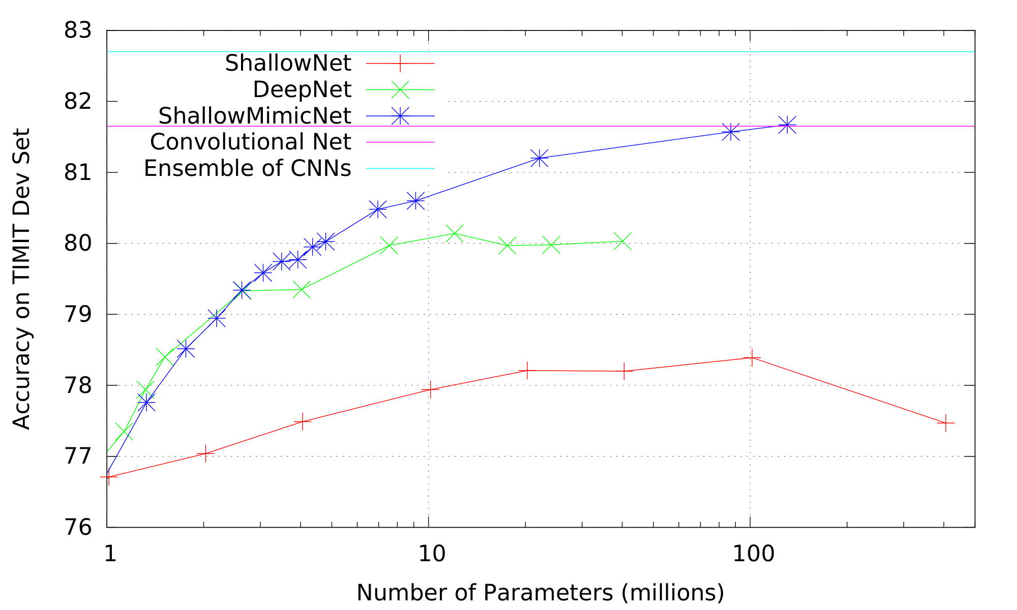
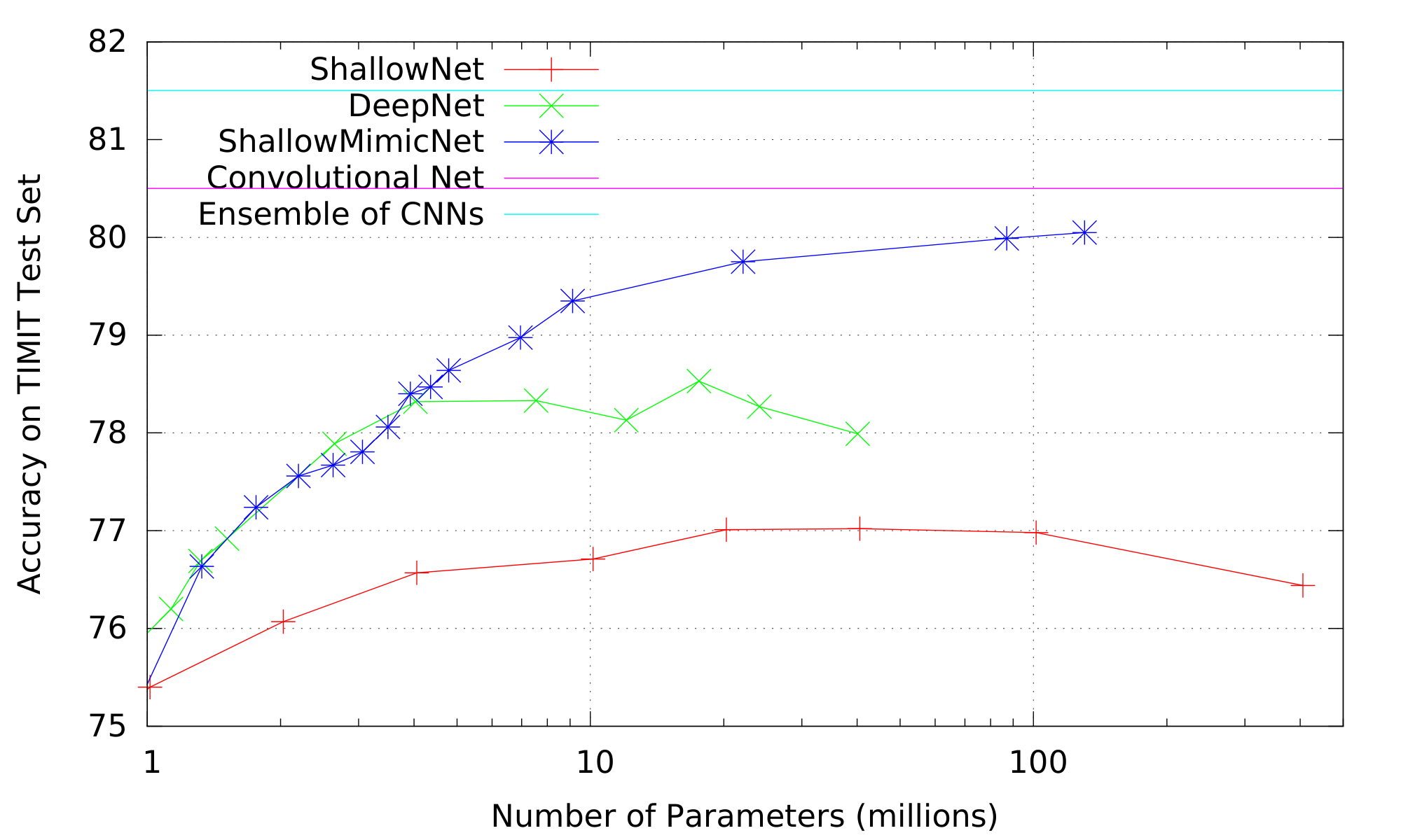
Figure 1: Accuracy of SNNs, DNNs, and Mimic SNNs vs. # of parameters on TIMIT Dev (left) and Test (right) sets. Accuracy of the CNN and target ECNN are shown as horizontal lines for reference. ::::

4. Object Recognition: CIFAR-10

Section Summary: The authors extended their model compression experiments from speech recognition to the CIFAR-10 image dataset, which contains 50,000 labeled 32x32 color photos across ten object categories, by adding a million unlabeled images from a larger collection for training. They used an ensemble of deep convolutional networks as a teacher to generate soft targets that train a much shallower mimic network containing just one convolutional layer plus fully connected units. This shallow mimic model reached accuracy levels comparable to prior deep convolutional nets on CIFAR-10, with further gains when trained on the ensemble, confirming that the compression approach generalizes beyond the original speech task.

To verify that the results on TIMIT generalize to other learning problems and task domains, we ran similar experiments on the CIFAR-10 Object Recognition Task [17]. CIFAR-10 consists of a set of natural images from 10 different object classes: airplane, automobile, bird, cat, deer, dog, frog, horse, ship, truck. The dataset is a labeled subset of the 80 million tiny images dataset [18] and is divided into 50, 000 train and 10, 000 test images. Each image is 32x32 pixels in 3 color channels, yielding input vectors with 3072 dimensions. We prepared the data by subtracting the mean and dividing the standard deviation of each image vector to perform global contrast normalization. We then applied ZCA whitening to the normalized images. This pre-processing is the same used in [19].

4.1 Learning to Mimic a Deep Convolutional Neural Network

Deep learning currently achieves state-of-the-art accuracies on many computer vision problems. The key to this success is deep convolutional nets with many alternating layers of convolutional, pooling and non-linear units. Recent advances such as dropout are also important to prevent over-fitting in these deep nets.

We follow the same approach as with TIMIT: An ensemble of deep CNN models is used to label CIFAR-10 images for model compression. The logit predictions from this teacher model are used as regression targets to train a mimic shallow neural net (SNN). CIFAR-10 images have a higher dimension than TIMIT (3072 vs. 1845), but the size of the CIFAR-10 training set is only 50, 000 compared to 1.1 million examples for TIMIT. Fortunately, unlike TIMIT, in CIFAR-10 we have access to unlabeled data from a similar distribution by using the super set of CIFAR-10: the 80 million tiny images dataset. We add the first 1 million images from the 80 million set to the original 50, 000 CIFAR-10 training images to create a 1.05M mimic training (transfer) set.

CIFAR-10 images are raw pixels for objects viewed from many different angles and positions, whereas TIMIT features are human-designed filter-bank features. In preliminary experiments we observed that non-convolutional nets do not perform well on CIFAR-10 no matter what their depth. Instead of raw pixels, the authors in [2] trained their shallow models on the SIFT features. Similarly, [7] used a base convolution and pooling layer to study different deep architectures. We follow the approach in [7] to allow our shallow models to benefit from convolution while keeping the models as shallow as possible, and introduce a single layer of convolution and pooling in our shallow mimic models to act as a feature extractor to create invariance to small translations in the pixel domain. The SNN-MIMIC models for CIFAR-10 thus consist of a convolution and max pooling layer followed by fully connected 1200 linear units and 30k non-linear units. As before, the linear units are there only to speed learning; they do not increase the model's representational power and can be absorbed into the weights in the non-linear layer after learning.

\begin{tabular}{|l|c|c|c|c|c|} \hline
 & \multirow{2}{*}{Architecture} & \multirow{2}{*}{# Param.} & \multirow{2}{*}{# Hidden units} & \multirow{2}{*}{Err.} \\
 & & & &\\ \hline \hline
  \multirow{2}{*}{DNN} & \multirow{2}{*}{2000-2000 + dropout} & \multirow{2}{*}{$\sim$ 10M} & \multirow{2}{*}{4k} & \multirow{2}{*}{57.8\%}
  \\ & & & & \\ \hline
  \multirow{2}{*}{SNN-30k} & 128c-p-1200L-30k & \multirow{2}{*}{$\sim$ 70M} & \multirow{2}{*}{$\sim$ 190k} & \multirow{2}{*}{21.8\%}
  \\ & + dropout input\&hidden & & & \\ \hline
  single-layer & 4000c-p & \multirow{2}{*}{$\sim$ 125M} & \multirow{2}{*}{$\sim$ 3.7B} & \multirow{2}{*}{18.4\%}
  \\ feature extraction & followed by SVM & & & \\ \hline
CNN [20] & 64c-p-64c-p-64c-p-16lc & \multirow{2}{*}{$\sim$ 10k}& \multirow{2}{*}{$\sim$ 110k} & \multirow{2}{*}{{15.6\%}}
  \\ (no augmentation) & + dropout on lc & & & \\ \hline 
CNN [21] & 64c-p-64c-p-128c-p-fc & \multirow{3}{*}{$\sim$ 56k}& \multirow{3}{*}{$\sim$ 120k} & \multirow{3}{*}{{15.13\%}}
  \\ (no augmentation) & + dropout on fc & & &
  \\ & and stochastic pooling & & & \\ \hline 
teacher CNN & 128c-p-128c-p-128c-p-1000fc & \multirow{3}{*}{$\sim$ 35k}& \multirow{3}{*}{$\sim$ 210k} & \multirow{3}{*}{\bf{12.0\%}}
  \\ (no augmentation) & + dropout on fc & & &
  \\ & and stochastic pooling & & & \\ \hline
ECNN & \multirow{2}{*}{ensemble of 4 CNNs} & \multirow{2}{*}{$\sim$ 140k}& \multirow{2}{*}{$\sim$ 840k} & {\bf{\multirow{2}{*}{11.0\%}}} 
  \\ (no augmentation) & & & & \\ \hline\hline
  SNN-CNN-MIMIC-30k & 64c-p-1200L-30k & \multirow{2}{*}{$\sim$ 54M} & \multirow{2}{*}{$\sim$ 110k} & \multirow{2}{*}{\bf{15.4\%}}
  \\ trained on a single CNN & with no regularization & & & \\ \hline
  SNN-CNN-MIMIC-30k & 128c-p-1200L-30k & \multirow{2}{*}{$\sim$ 70M} & \multirow{2}{*}{$\sim$ 190k} & \multirow{2}{*}{\bf{15.1\%}}
  \\ trained on a single CNN & with no regularization & & & \\ \hline
  SNN-ECNN-MIMIC-30k & 128c-p-1200L-30k & \multirow{2}{*}{$\sim$ 70M} & \multirow{2}{*}{$\sim$ 190k} & \multirow{2}{*}{\bf{14.2\%}}
  \\ trained on ensemble& with no regularization & & & \\\hline
\end{tabular}

Results on CIFAR-10 are consistent with those from TIMIT. Table 2 shows results for the shallow mimic models, and for much-deeper convolutional nets. The shallow mimic net trained to mimic the teacher CNN (SNN-CNN-MIMIC-30k) achieves accuracy comparable to CNNs with multiple convolutional and pooling layers. And by training the shallow model to mimic the ensemble of CNNs (SNN-ECNN-MIMIC-30k), accuracy is improved an additional 0.9%. The mimic models are able to achieve accuracies previously unseen on CIFAR-10 with models with so few layers. Although the deep convolution nets have more hidden units than the shallow mimic models, because of weight sharing, the deeper nets with multiple convolution layers have fewer parameters than the shallow fully-connected mimic models. Still, it is surprising to see how accurate the shallow mimic models are, and that their performance continues to improve as the performance of the teacher model improves (see further discussion of this in Section 5.2).

5. Discussion

Section Summary: Mimic models can outperform those trained directly on original labels because the teacher networks effectively regularize the data by correcting errors, simplifying hard-to-learn patterns, and supplying informative soft probabilities rather than rigid zero-one targets. Experiments further show that shallow networks possess ample capacity to match or approach deep-model accuracy when given sufficiently strong teachers, implying that their main shortfall lies in training methods rather than inherent limits. In addition, these shallower architectures train and run much faster on parallel hardware, completing inference in just a few steps instead of the many sequential layers required by deep networks.

5.1 Why Mimic Models Can Be More Accurate than Training on Original Labels

It may be surprising that models trained on the prediction targets taken from other models can be more accurate than models trained on the original labels. There are a variety of reasons why this can happen:

• if some labels have errors, the teacher model may eliminate some of these errors (i.e., censor the data), thus making learning easier for the student: on TIMIT, there are mislabeled frames introduced by the HMM forced-alignment procedure.
• if there are regions in the $p(y|X)$ that are difficult to learn given the features, sample density, and function complexity, the teacher may provide simpler, soft labels to the student. The complexity in the data set has been washed away by filtering the targets through the teacher model.
• learning from the original hard 0/1 labels can be more difficult than learning from the teacher's conditional probabilities: on TIMIT only one of 183 outputs is non-zero on each training case, but the mimic model sees non-zero targets for most outputs on most training cases. Moreover, the teacher model can spread the uncertainty over multiple outputs when it is not confident of its prediction. Yet, the teacher model can concentrate the probability mass on one (or few) outputs on easy cases. The uncertainty from the teacher model is far more informative to guiding the student model than the original 0/1 labels. This benefit appears to be further enhanced by training on logits.

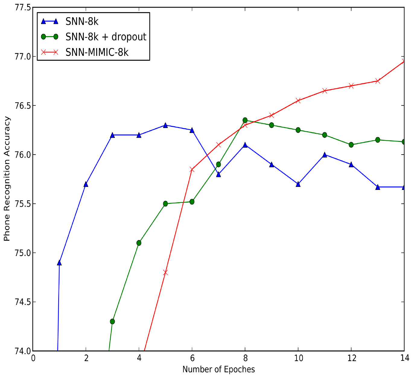
The mechanisms above can be seen as forms of regularization that help prevent overfitting in the student model. Shallow models trained on the original targets are more prone to overfitting than deep models—they begin to overfit before learning the accurate functions learned by deeper models even with dropout (see Figure 2). If we had more effective regularization methods for shallow models, some of the performance gap between shallow and deep models might disappear. Model compression appears to be a form of regularization that is effective at reducing this gap.

5.2 The Capacity and Representational Power of Shallow Models

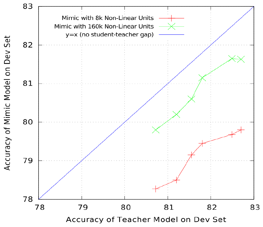
Figure 3 shows results of an experiment with TIMIT where we trained shallow mimic models of two sizes (SNN-MIMIC-8k and SNN-MIMIC-160k) on teacher models of different accuracies. The two shallow mimic models are trained on the same number of data points. The only difference between them is the size of the hidden layer. The x-axis shows the accuracy of the teacher model, and the y-axis is the accuracy of the mimic models. Lines parallel to the diagonal suggest that increases in the accuracy of the teacher models yield similar increases in the accuracy of the mimic models. Although the data does not fall perfectly on a diagonal, there is strong evidence that the accuracy of the mimic models continues to increase as the accuracy of the teacher model improves, suggesting that the mimic models are not (yet) running out of capacity. When training on the same targets, SNN-MIMIC-8k always perform worse than SNN-MIMIC-160K that has 10 times more parameters. Although there is a consistent performance gap between the two models due to the difference in size, the smaller shallow model was eventually able to achieve a performance comparable to the larger shallow net by learning from a better teacher, and the accuracy of both models continues to increase as teacher accuracy increases. This suggests that shallow models with a number of parameters comparable to deep models are likely capable of learning even more accurate functions if a more accurate teacher and/or more unlabeled data became available. Similarly, on CIFAR-10 we saw that increasing the accuracy of the teacher model by forming an ensemble of deep CNNs yielded commensurate increase in the accuracy of the student model. We see little evidence that shallow models have limited capacity or representational power. Instead, the main limitation appears to be the learning and regularization procedures used to train the shallow models.

5.3 Parallel Distributed Processing vs. Deep Sequential Processing

Our results show that shallow nets can be competitive with deep models on speech and vision tasks. One potential benefit of shallow nets is that training them scales well with the modern parallel hardware. In our experiments the deep models usually required 8–12 hours to train on Nvidia GTX 580 GPUs to reach the state-of-the-art performance on TIMIT and CIFAR-10 datasets. Although some of the shallow mimic models have more parameters than the deep models, the shallow models train much faster and reach similar accuracies in only 1–2 hours.

Also, given parallel computational resources, at run-time shallow models can finish computation in 2 or 3 cycles for a given input, whereas a deep architecture has to make sequential inference through each of its layers, expending a number of cycles proportional to the depth of the model. This benefit can be important in on-line inference settings where data parallelization is not as easy to achieve as it is in the batch inference setting. For real-time applications such as surveillance or real-time speech translation, a model that responds in fewer cycles can be beneficial.

6. Future Work

Section Summary: The authors plan to label a dataset of 80 million tiny images using a high-performing teacher model, then use those labels to train very simple shallow networks that try to match the behavior of deep convolutional models. They also note that the mimicry approach could have practical value by letting smaller, faster student models reach the accuracy of large deep networks or ensembles, while allowing flexible trade-offs between speed and performance. Finally, they suggest that future algorithms should aim to train accurate shallow models directly from data, rather than requiring an intermediate teacher or massive unlabeled sets.

The tiny images dataset contains 80 millions images. We are currently investigating if by labeling these 80M images with a teacher, it is possible to train shallow models with no convolutional or pooling layers to mimic deep convolutional models.

This paper focused on training the shallowest-possible models to mimic deep models in order to better understand the importance of model depth in learning. As suggested in Section 5.3, there are practical applications of this work as well: student models of small-to-medium size and depth can be trained to mimic very large, high accuracy deep models, and ensembles of deep models, thus yielding better accuracy with reduced runtime cost than is currently achievable without model compression. This approach allows one to adjust flexibly the trade-off between accuracy and computational cost.

In this paper we are able to demonstrate empirically that shallow models can, at least in principle, learn more accurate functions without a large increase in the number of parameters. The algorithm we use to do this—training the shallow model to mimic a more accurate deep model, however, is awkward. It depends on the availability of either a large unlabeled data set (to reduce the gap between teacher and mimic model) or a teacher model of very high accuracy, or both. Developing algorithms to train shallow models of high accuracy directly from the original data without going through the intermediate teacher model would, if possible, be a significant contribution.

7. Conclusions

Section Summary: Experiments show that simple, shallow neural networks can reach the same accuracy as complex deep models on standard speech and image recognition benchmarks. By training these single-layer networks to imitate deeper ones, researchers achieved comparable results to sophisticated convolutional architectures. The findings indicate that depth may mainly help with current training methods rather than being strictly necessary, suggesting that better algorithms could make shallower networks just as effective.

We demonstrate empirically that shallow neural nets can be trained to achieve performances previously achievable only by deep models on the TIMIT phoneme recognition and CIFAR-10 image recognition tasks. Single-layer fully-connected feedforward nets trained to mimic deep models can perform similarly to well-engineered complex deep convolutional architectures. The results suggest that the strength of deep learning may arise in part from a good match between deep architectures and current training procedures, and that it may be possible to devise better learning algorithms to train more accurate shallow feed-forward nets. For a given number of parameters, depth may make learning easier, but may not always be essential.

Acknowledgements We thank Li Deng for generous help with TIMIT, Li Deng and Ossama Abdel-Hamid for code for the TIMIT convolutional model, Chris Burges, Li Deng, Ran Gilad-Bachrach, Tapas Kanungo and John Platt for discussion that significantly improved this work, and Mike Aultman for help with the GPU cluster.

References

Section Summary: This section provides a numbered list of 21 academic citations, primarily from conferences and journals in computer science and machine learning. The referenced works focus on neural network methods, including deep learning architectures, speech recognition models, and techniques for improving efficiency and training. They represent key prior research that supports the paper's discussion of related technical developments.

[1] Ossama Abdel-Hamid, Abdel-rahman Mohamed, Hui Jiang, and Gerald Penn. Applying convolutional neural networks concepts to hybrid nn-hmm model for speech recognition. In Acoustics, Speech and Signal Processing (ICASSP), 2012 IEEE International Conference on, pages 4277–4280. IEEE, 2012.

[2] Yann N Dauphin and Yoshua Bengio. Big neural networks waste capacity. arXiv preprint arXiv:1301.3583, 2013.

[3] Dumitru Erhan, Yoshua Bengio, Aaron Courville, Pierre-Antoine Manzagol, Pascal Vincent, and Samy Bengio. Why does unsupervised pre-training help deep learning? The Journal of Machine Learning Research, 11:625–660, 2010.

[4] G.E. Hinton and R.R. Salakhutdinov. Reducing the dimensionality of data with neural networks. Science, 313(5786):504–507, 2006.

[5] P. Vincent, H. Larochelle, I. Lajoie, Y. Bengio, and P.A. Manzagol. Stacked denoising autoencoders: Learning useful representations in a deep network with a local denoising criterion. The Journal of Machine Learning Research, 11:3371–3408, 2010.

[6] George Cybenko. Approximation by superpositions of a sigmoidal function. Mathematics of control, signals and systems, 2(4):303–314, 1989.

[7] David Eigen, Jason Rolfe, Rob Fergus, and Yann LeCun. Understanding deep architectures using a recursive convolutional network. arXiv preprint arXiv:1312.1847, 2013.

[8] Frank Seide, Gang Li, and Dong Yu. Conversational speech transcription using context-dependent deep neural networks. In Interspeech, pages 437–440, 2011.

[9] Cristian Buciluǎ, Rich Caruana, and Alexandru Niculescu-Mizil. Model compression. In Proceedings of the 12th ACM SIGKDD international conference on Knowledge discovery and data mining, pages 535–541. ACM, 2006.

[10] Tara N Sainath, Brian Kingsbury, Vikas Sindhwani, Ebru Arisoy, and Bhuvana Ramabhadran. Low-rank matrix factorization for deep neural network training with high-dimensional output targets. In Acoustics, Speech and Signal Processing (ICASSP), 2013 IEEE International Conference on, pages 6655–6659. IEEE, 2013.

[11] Jian Xue, Jinyu Li, and Yifan Gong. Restructuring of deep neural network acoustic models with singular value decomposition. Proc. Interspeech, Lyon, France, 2013.

[12] K-F Lee and H-W Hon. Speaker-independent phone recognition using hidden markov models. Acoustics, Speech and Signal Processing, IEEE Transactions on, 37(11):1641–1648, 1989.

[13] Abdel-rahman Mohamed, George E Dahl, and Geoffrey Hinton. Acoustic modeling using deep belief networks. Audio, Speech, and Language Processing, IEEE Transactions on, 20(1):14–22, 2012.

[14] V. Nair and G.E. Hinton. Rectified linear units improve restricted boltzmann machines. In Proc. 27th International Conference on Machine Learning, pages 807–814. Omnipress Madison, WI, 2010.

[15] Ossama Abdel-Hamid, Li Deng, and Dong Yu. Exploring convolutional neural network structures and optimization techniques for speech recognition. Interspeech 2013, 2013.

[16] Li Deng, Jinyu Li, Jui-Ting Huang, Kaisheng Yao, Dong Yu, Frank Seide, Michael Seltzer, Geoff Zweig, Xiaodong He, Jason Williams, et al. Recent advances in deep learning for speech research at microsoft. ICASSP 2013, 2013.

[17] Alex Krizhevsky and Geoffrey Hinton. Learning multiple layers of features from tiny images. Computer Science Department, University of Toronto, Tech. Rep, 2009.

[18] Antonio Torralba, Robert Fergus, and William T Freeman. 80 million tiny images: A large data set for nonparametric object and scene recognition. Pattern Analysis and Machine Intelligence, IEEE Transactions on, 30(11):1958–1970, 2008.

[19] Ian Goodfellow, David Warde-Farley, Mehdi Mirza, Aaron Courville, and Yoshua Bengio. Maxout networks. In Proceedings of The 30th International Conference on Machine Learning, pages 1319–1327, 2013.

[20] G.E. Hinton, N. Srivastava, A. Krizhevsky, I. Sutskever, and R.R. Salakhutdinov. Improving neural networks by preventing co-adaptation of feature detectors. arXiv preprint arXiv:1207.0580, 2012.

[21] Matthew D Zeiler and Rob Fergus. Stochastic pooling for regularization of deep convolutional neural networks. arXiv preprint arXiv:1301.3557, 2013.