Semi-Supervised Classification with Graph Convolutional Networks

Thomas N. Kipf
University of Amsterdam
[email protected]

Max Welling
University of Amsterdam
Canadian Institute for Advanced Research (CIFAR)
[email protected]

Abstract

We present a scalable approach for semi-supervised learning on graph-structured data that is based on an efficient variant of convolutional neural networks which operate directly on graphs. We motivate the choice of our convolutional architecture via a localized first-order approximation of spectral graph convolutions. Our model scales linearly in the number of graph edges and learns hidden layer representations that encode both local graph structure and features of nodes. In a number of experiments on citation networks and on a knowledge graph dataset we demonstrate that our approach outperforms related methods by a significant margin.

Executive Summary: In today's data-driven world, many real-world problems involve networks where entities connect in complex ways, such as academic papers linked by citations or entities in knowledge bases connected by relationships. Classifying these entities—determining their categories or types—is challenging because labeling examples is costly and time-consuming, often leaving only a tiny fraction of data annotated. Traditional machine learning struggles here, as it overlooks the rich structure of these connections, which can help predict labels for unlabeled items by propagating information from nearby ones. This issue is pressing now, as graph-structured data explodes in fields like social media analysis, recommendation systems, and scientific research, demanding efficient tools to leverage limited labels without massive human effort.

This paper aims to develop and test a new method for classifying nodes in graphs using semi-supervised learning, where a small set of labeled examples guides predictions for the rest. It demonstrates how to build a graph convolutional network (GCN), a type of neural network adapted for graphs, to learn node representations that incorporate both node features and their connections.

The authors created a simple, multi-layer GCN model that processes graph data directly. Drawing from spectral graph theory—a way to analyze graphs via mathematical filters—they simplified it into an efficient approximation that aggregates information from a node's immediate neighbors in each layer. This avoids heavy computations like full eigenvector breakdowns, scaling linearly with the number of connections (edges) in the graph. They tested it on three citation network datasets (Citeseer, Cora, Pubmed) with thousands of documents and sparse word features, plus a knowledge graph dataset (NELL) with over 65,000 nodes representing entities and relations. Experiments used just 20 labels per class for citation data (about 3-5% of nodes) and one label per class for NELL (0.1%), training via standard optimization techniques over 200 iterations, with a focus on two-layer models for balance.

The GCN achieved top results across datasets. On Cora, it reached 81.5% classification accuracy, surpassing the next-best method (Planetoid) by about 6 percentage points; similar gains appeared on Citeseer (70.3% vs. 64.7%) and Pubmed (79.0% vs. 77.2%), and on NELL (66.0% vs. 61.9%). It also ran faster, taking 4-48 seconds per dataset versus 13-185 seconds for Planetoid, thanks to its linear scaling. A key tweak, called the renormalization trick, boosted accuracy by 1-2 points over simpler variants and prevented training instability in deeper models. Random splits confirmed robustness, with accuracies within 1-2 points of fixed benchmarks.

These findings mean GCNs can dramatically improve classification in graph settings by embedding both structure and features into compact node representations, reducing reliance on labels and cutting compute costs. This matters for practical applications: in research networks, it speeds up topic categorization; in knowledge graphs, it enhances entity recognition with minimal supervision, potentially saving resources in AI systems for search or drug discovery. Unlike prior methods that assume edges only signal similarity or require multi-step pipelines, GCNs learn flexibly, outperforming expectations on diverse graphs and enabling deeper models for richer insights—though it slightly underperforms on some baselines without graph structure.

Leaders should prioritize integrating GCNs into graph-based AI pipelines for semi-supervised tasks, starting with citation or social network pilots to classify nodes efficiently. For larger scales, implement mini-batch training to handle graphs beyond GPU memory. Explore variants for directed edges or weighted connections, weighing trade-offs like added complexity against gains in domains like web graphs. Before full rollout, validate on domain-specific data.

The model assumes undirected graphs and local neighborhoods up to a few hops, which may miss long-range dependencies in sparse or directed networks; memory needs grow with edges, limiting very large graphs without approximations. Confidence is high for medium-sized undirected graphs (thousands of nodes), backed by consistent wins over state-of-the-art baselines, but caution applies to highly irregular structures where further tuning might be needed.

1. Introduction

Section Summary: The paper addresses the challenge of classifying nodes such as documents in a graph like a citation network, when labels are available for only a small number of nodes. Traditional approaches rely on explicit regularization terms that encourage connected nodes to share similar labels, but this can limit flexibility since edges may carry richer information. The authors instead propose a neural network model that directly incorporates the graph structure through its layers, training solely on the available labeled data to learn useful representations for all nodes and achieve strong performance in both accuracy and speed.

We consider the problem of classifying nodes (such as documents) in a graph (such as a citation network), where labels are only available for a small subset of nodes. This problem can be framed as graph-based semi-supervised learning, where label information is smoothed over the graph via some form of explicit graph-based regularization ([1, 2, 3, 4]), e.g. by using a graph Laplacian regularization term in the loss function:

$ \mathcal{L} = \mathcal{L}0 + \lambda \mathcal{L}{\text{reg}}, , \quad \text{with} \quad \mathcal{L}{\text{reg}}= \sum{i, j}A_{ij}\Vert f(X_i)-f(X_j) \Vert ^2 = f(X)^\top \Delta f(X) , .\tag{1} $

Here, $\mathcal{L}0$ denotes the supervised loss w.r.t. the labeled part of the graph, $f(\cdot)$ can be a neural network-like differentiable function, $\lambda$ is a weighing factor and $X$ is a matrix of node feature vectors $X_i$. $\Delta = D - A$ denotes the unnormalized graph Laplacian of an undirected graph $\mathcal{G}=(\mathcal{V}, \mathcal{E})$ with $N$ nodes $v_i \in \mathcal{V}$, edges $(v_i, v_j)\in\mathcal{E}$, an adjacency matrix $A\in\mathbb{R}^{N\times N}$ (binary or weighted) and a degree matrix $D{ii} = \sum_j A_{ij}$. The formulation of Eq.@ Equation 1 relies on the assumption that connected nodes in the graph are likely to share the same label. This assumption, however, might restrict modeling capacity, as graph edges need not necessarily encode node similarity, but could contain additional information.

In this work, we encode the graph structure directly using a neural network model $f(X, A)$ and train on a supervised target $\mathcal{L}_0$ for all nodes with labels, thereby avoiding explicit graph-based regularization in the loss function. Conditioning $f(\cdot)$ on the adjacency matrix of the graph will allow the model to distribute gradient information from the supervised loss $\mathcal{L}_0$ and will enable it to learn representations of nodes both with and without labels.

Our contributions are two-fold. Firstly, we introduce a simple and well-behaved layer-wise propagation rule for neural network models which operate directly on graphs and show how it can be motivated from a first-order approximation of spectral graph convolutions ([5]). Secondly, we demonstrate how this form of a graph-based neural network model can be used for fast and scalable semi-supervised classification of nodes in a graph. Experiments on a number of datasets demonstrate that our model compares favorably both in classification accuracy and efficiency (measured in wall-clock time) against state-of-the-art methods for semi-supervised learning.

2. Fast Approximate Convolutions on Graphs

Section Summary: This section motivates a practical graph convolutional network by deriving its layer-wise update rule from spectral graph theory. It starts from frequency-domain filters defined via the eigenvectors of the graph Laplacian, then uses a first-order Chebyshev approximation (with further simplifications such as setting the largest eigenvalue to 2) to obtain cheap, localized operations that depend only on immediate neighbors. The resulting propagation rule renormalizes the adjacency matrix with added self-loops, allowing efficient multi-layer models that avoid costly eigendecompositions while still capturing neighborhood structure.

In this section, we provide theoretical motivation for a specific graph-based neural network model $f(X, A)$ that we will use in the rest of this paper. We consider a multi-layer Graph Convolutional Network (GCN) with the following layer-wise propagation rule:

$ \textstyle H^{(l+1)}= \sigma!\left(\tilde{D}^{-\frac{1}{2}} \tilde{A}\tilde{D}^{-\frac{1}{2}}H^{(l)} W^{(l)} \right) , .\tag{2} $

Here, $\tilde{A} = A + I_N$ is the adjacency matrix of the undirected graph $\mathcal{G}$ with added self-connections. $I_N$ is the identity matrix, $\tilde{D}{ii} = \sum_j \tilde{A}{ij}$ and $W^{(l)}$ is a layer-specific trainable weight matrix. $\sigma(\cdot)$ denotes an activation function, such as the $\mathrm{ReLU}(\cdot) = \max(0, \cdot)$. $H^{(l)}\in \mathbb{R}^{N\times D}$ is the matrix of activations in the $l^{\text{th}}$ layer; $H^{(0)}=X$. In the following, we show that the form of this propagation rule can be motivated[^1] via a first-order approximation of localized spectral filters on graphs ([5, 6]).

[^1]: We provide an alternative interpretation of this propagation rule based on the Weisfeiler-Lehman algorithm ([7]) in Appendix A.

2.1 Spectral Graph Convolutions

We consider spectral convolutions on graphs defined as the multiplication of a signal $x\in \mathbb{R}^N$ (a scalar for every node) with a filter $g_{\theta}=\text{diag}(\theta)$ parameterized by $\theta\in \mathbb{R}^N$ in the Fourier domain, i.e.:

$ g_{\theta} \star x = Ug_{\theta}U^\top x , ,\tag{3} $

where $U$ is the matrix of eigenvectors of the normalized graph Laplacian $L = I_N - D^{-\frac{1}{2}}AD^{-\frac{1}{2}} = U\Lambda U^\top$, with a diagonal matrix of its eigenvalues $\Lambda$ and $U^\top x$ being the graph Fourier transform of $x$. We can understand $g_{\theta}$ as a function of the eigenvalues of $L$, i.e. $g_{\theta}(\Lambda)$. Evaluating Eq.@ Equation 3 is computationally expensive, as multiplication with the eigenvector matrix $U$ is $\mathcal{O}(N^2)$. Furthermore, computing the eigendecomposition of $L$ in the first place might be prohibitively expensive for large graphs. To circumvent this problem, it was suggested in [5] that $g_{\theta}(\Lambda)$ can be well-approximated by a truncated expansion in terms of Chebyshev polynomials $T_k(x)$ up to $K^{\text{th}}$ order:

$ g_{\theta'}(\Lambda) \approx \sum_{k=0}^{K} \theta_k ' T_k(\tilde{\Lambda}) , ,\tag{4} $

with a rescaled $\tilde{\Lambda}=\frac{2}{\lambda_{\text{max}}}\Lambda-I_N$. $\lambda_{\text{max}}$ denotes the largest eigenvalue of $L$. $\theta'\in \mathbb{R}^K$ is now a vector of Chebyshev coefficients. The Chebyshev polynomials are recursively defined as $T_k(x) = 2xT_{k-1}(x) - T_{k-2}(x)$, with $T_0(x)=1$ and $T_1(x)=x$. The reader is referred to [5] for an in-depth discussion of this approximation.

Going back to our definition of a convolution of a signal $x$ with a filter $g_{\theta'}$, we now have:

$ g_{\theta'} \star x \approx \sum_{k=0}^{K} \theta_k' T_k(\tilde{L}) x , ,\tag{5} $

with $\tilde{L} = \frac{2}{\lambda_{\text{max}}}L-I_N$; as can easily be verified by noticing that $(U\Lambda U^\top)^k = U \Lambda^k U^\top$. Note that this expression is now $K$-localized since it is a $K^{\text{th}}$-order polynomial in the Laplacian, i.e. it depends only on nodes that are at maximum $K$ steps away from the central node ($K^{\text{th}}$-order neighborhood). The complexity of evaluating Eq.@ Equation 5 is $\mathcal{O}(|\mathcal{E}|)$, i.e. linear in the number of edges. [6] use this $K$-localized convolution to define a convolutional neural network on graphs.

2.2 Layer-Wise Linear Model

A neural network model based on graph convolutions can therefore be built by stacking multiple convolutional layers of the form of Eq.@ Equation 5, each layer followed by a point-wise non-linearity. Now, imagine we limited the layer-wise convolution operation to $K=1$ (see Eq.@ Equation 5), i.e. a function that is linear w.r.t. $L$ and therefore a linear function on the graph Laplacian spectrum.

In this way, we can still recover a rich class of convolutional filter functions by stacking multiple such layers, but we are not limited to the explicit parameterization given by, e.g., the Chebyshev polynomials. We intuitively expect that such a model can alleviate the problem of overfitting on local neighborhood structures for graphs with very wide node degree distributions, such as social networks, citation networks, knowledge graphs and many other real-world graph datasets. Additionally, for a fixed computational budget, this layer-wise linear formulation allows us to build deeper models, a practice that is known to improve modeling capacity on a number of domains ([8]).

In this linear formulation of a GCN we further approximate $\lambda_{\text{max}}\approx 2$, as we can expect that neural network parameters will adapt to this change in scale during training. Under these approximations Eq.@ Equation 5 simplifies to:

$ g_{\theta'} \star x \approx \theta_0' x

• \theta_1' \left(L-I_N\right)x = \theta_0' x - \theta_1' D^{-\frac{1}{2}}AD^{-\frac{1}{2}} x , ,\tag{6} $

with two free parameters $\theta_0'$ and $\theta_1'$. The filter parameters can be shared over the whole graph. Successive application of filters of this form then effectively convolve the $k^{\text{th}}$-order neighborhood of a node, where $k$ is the number of successive filtering operations or convolutional layers in the neural network model.

In practice, it can be beneficial to constrain the number of parameters further to address overfitting and to minimize the number of operations (such as matrix multiplications) per layer. This leaves us with the following expression:

$ g_{\theta} \star x \approx \theta \left(I_N + D^{-\frac{1}{2}}AD^{-\frac{1}{2}}\right) x , ,\tag{7} $

with a single parameter $\theta = \theta_0'=-\theta_1'$. Note that $I_N + D^{-\frac{1}{2}}AD^{-\frac{1}{2}}$ now has eigenvalues in the range $[0, 2]$. Repeated application of this operator can therefore lead to numerical instabilities and exploding/vanishing gradients when used in a deep neural network model. To alleviate this problem, we introduce the following renormalization trick: $I_N + D^{-\frac{1}{2}}AD^{-\frac{1}{2}}\rightarrow \tilde{D}^{-\frac{1}{2}}\tilde{A}\tilde{D}^{-\frac{1}{2}}$, with $\tilde{A} = A + I_N$ and $\tilde{D}{ii} = \sum_j \tilde{A}{ij}$.

We can generalize this definition to a signal $X\in\mathbb{R}^{N\times C}$ with $C$ input channels (i.e. a $C$-dimensional feature vector for every node) and $F$ filters or feature maps as follows:

$ Z = \tilde{D}^{-\frac{1}{2}}\tilde{A}\tilde{D}^{-\frac{1}{2}}X\Theta , ,\tag{8} $

where $\Theta\in\mathbb{R}^{C\times F}$ is now a matrix of filter parameters and $Z\in\mathbb{R}^{N\times F}$ is the convolved signal matrix. This filtering operation has complexity $\mathcal{O}(|\mathcal{E}|FC)$, as $\tilde{A}X$ can be efficiently implemented as a product of a sparse matrix with a dense matrix.

3. Semi-Supervised Node Classification

Section Summary: The section describes how a graph convolutional network can perform semi-supervised node classification by combining node feature data with the underlying graph structure encoded in the adjacency matrix. This approach is especially useful when the graph connections, such as citations or relations, carry information absent from the features alone. The authors present a simple two-layer model that propagates information through normalized adjacency multiplications and nonlinear activations, trains via cross-entropy loss on the few labeled nodes using gradient descent, and achieves linear computational cost in the number of edges.

Having introduced a simple, yet flexible model $f(X, A)$ for efficient information propagation on graphs, we can return to the problem of semi-supervised node classification. As outlined in the introduction, we can relax certain assumptions typically made in graph-based semi-supervised learning by conditioning our model $f(X, A)$ both on the data $X$ and on the adjacency matrix $A$ of the underlying graph structure. We expect this setting to be especially powerful in scenarios where the adjacency matrix contains information not present in the data $X$, such as citation links between documents in a citation network or relations in a knowledge graph. The overall model, a multi-layer GCN for semi-supervised learning, is schematically depicted in Figure 1.

3.1 Example

In the following, we consider a two-layer GCN for semi-supervised node classification on a graph with a symmetric adjacency matrix $A$ (binary or weighted). We first calculate $\hat{A} = \tilde{D}^{-\frac{1}{2}}\tilde{A}\tilde{D}^{-\frac{1}{2}}$ in a pre-processing step. Our forward model then takes the simple form:

$ Z= f(X, A) = \mathrm{softmax}!\left(\hat{A} , , \mathrm{ReLU}!\left(\hat{A} X W^{(0)} \right) W^{(1)} \right) , .\tag{9} $

Here, $W^{(0)}\in \mathbb{R}^{C\times H}$ is an input-to-hidden weight matrix for a hidden layer with $H$ feature maps. $W^{(1)}\in \mathbb{R}^{H\times F}$ is a hidden-to-output weight matrix. The softmax activation function, defined as $\mathrm{softmax}(x_i)=\frac{1}{\mathcal{Z}}\exp(x_i)$ with $\mathcal{Z}=\sum_i \exp(x_i)$, is applied row-wise. For semi-supervised multi-class classification, we then evaluate the cross-entropy error over all labeled examples:

$ \mathcal{L}= -\sum_{l\in\mathcal{Y}L}\sum{f=1}^F Y_{lf} \ln Z_{lf} , ,\tag{10} $

where $\mathcal{Y}_L$ is the set of node indices that have labels.

The neural network weights $W^{(0)}$ and $W^{(1)}$ are trained using gradient descent. In this work, we perform batch gradient descent using the full dataset for every training iteration, which is a viable option as long as datasets fit in memory. Using a sparse representation for $A$, memory requirement is $\mathcal{O}(|\mathcal{E}|)$, i.e. linear in the number of edges. Stochasticity in the training process is introduced via dropout ([11]). We leave memory-efficient extensions with mini-batch stochastic gradient descent for future work.

3.2 Implementation

In practice, we make use of TensorFlow ([12]) for an efficient GPU-based implementation[^2] of Eq.@ Equation 9 using sparse-dense matrix multiplications. The computational complexity of evaluating Eq.@ Equation 9 is then $\mathcal{O}(|\mathcal{E}|CHF)$, i.e. linear in the number of graph edges.

[^2]: Code to reproduce our experiments is available at https://github.com/tkipf/gcn.

4. Related Work

Section Summary: The section reviews prior work in two areas that inform the authors' graph-based neural network model. It first covers graph-based semi-supervised learning, which includes older methods relying on graph Laplacian regularization such as label propagation, as well as newer embedding techniques like DeepWalk and node2vec that generate node representations from random walks before separate training steps. It then discusses neural networks designed for graph data, noting early recurrent approaches and spectral convolutional methods, while highlighting limitations in scalability that the authors address through simplifications for large-scale node classification tasks.

Our model draws inspiration both from the field of graph-based semi-supervised learning and from recent work on neural networks that operate on graphs. In what follows, we provide a brief overview on related work in both fields.

4.1 Graph-Based Semi-Supervised Learning

A large number of approaches for semi-supervised learning using graph representations have been proposed in recent years, most of which fall into two broad categories: methods that use some form of explicit graph Laplacian regularization and graph embedding-based approaches. Prominent examples for graph Laplacian regularization include label propagation ([1]), manifold regularization ([3]) and deep semi-supervised embedding ([4]).

Recently, attention has shifted to models that learn graph embeddings with methods inspired by the skip-gram model ([13]). DeepWalk ([14]) learns embeddings via the prediction of the local neighborhood of nodes, sampled from random walks on the graph. LINE ([15]) and node2vec ([16]) extend DeepWalk with more sophisticated random walk or breadth-first search schemes. For all these methods, however, a multi-step pipeline including random walk generation and semi-supervised training is required where each step has to be optimized separately. Planetoid ([17]) alleviates this by injecting label information in the process of learning embeddings.

4.2 Neural Networks on Graphs

Neural networks that operate on graphs have previously been introduced in [18, 19] as a form of recurrent neural network. Their framework requires the repeated application of contraction maps as propagation functions until node representations reach a stable fixed point. This restriction was later alleviated in [20] by introducing modern practices for recurrent neural network training to the original graph neural network framework. [21] introduced a convolution-like propagation rule on graphs and methods for graph-level classification. Their approach requires to learn node degree-specific weight matrices which does not scale to large graphs with wide node degree distributions. Our model instead uses a single weight matrix per layer and deals with varying node degrees through an appropriate normalization of the adjacency matrix (see Section 3.1).

A related approach to node classification with a graph-based neural network was recently introduced in [22]. They report $\mathcal{O}(N^2)$ complexity, limiting the range of possible applications. In a different yet related model, [23] convert graphs locally into sequences that are fed into a conventional 1D convolutional neural network, which requires the definition of a node ordering in a pre-processing step.

Our method is based on spectral graph convolutional neural networks, introduced in [24] and later extended by [6] with fast localized convolutions. In contrast to these works, we consider here the task of transductive node classification within networks of significantly larger scale. We show that in this setting, a number of simplifications (see Section 2.2) can be introduced to the original frameworks of [24] and [6] that improve scalability and classification performance in large-scale networks.

5. Experiments

Section Summary: The experiments evaluate a graph convolutional network on semi-supervised classification tasks using citation networks such as Cora, Citeseer, and Pubmed, along with a large knowledge-graph dataset called NELL, plus timing tests on synthetic random graphs of varying sizes. Models are trained with a fixed two-layer architecture and standard optimization settings, using small numbers of labeled examples per class while leveraging all node features and the graph structure. Performance is compared against several established baselines including label propagation, manifold regularization, DeepWalk embeddings, iterative classification, and Planetoid.

We test our model in a number of experiments: semi-supervised document classification in citation networks, semi-supervised entity classification in a bipartite graph extracted from a knowledge graph, an evaluation of various graph propagation models and a run-time analysis on random graphs.

5.1 Datasets

We closely follow the experimental setup in [17]. Dataset statistics are summarized in Table 1. In the citation network datasets—Citeseer, Cora and Pubmed ([10])—nodes are documents and edges are citation links. Label rate denotes the number of labeled nodes that are used for training divided by the total number of nodes in each dataset. NELL ([25, 17]) is a bipartite graph dataset extracted from a knowledge graph with 55, 864 relation nodes and 9, 891 entity nodes.

: Table 1: Dataset statistics, as reported in [17].

Dataset	Type	Nodes	Edges	Classes	Features	Label rate
Citeseer	Citation network	3, 327	4, 732	$6$	3, 703	$0.036$
Cora	Citation network	2, 708	5, 429	$7$	1, 433	$0.052$
Pubmed	Citation network	19, 717	44, 338	$3$	500	$0.003$
NELL	Knowledge graph	65, 755	266, 144	$210$	5, 414	$0.001$

Citation networks

We consider three citation network datasets: Citeseer, Cora and Pubmed ([10]). The datasets contain sparse bag-of-words feature vectors for each document and a list of citation links between documents. We treat the citation links as (undirected) edges and construct a binary, symmetric adjacency matrix $A$. Each document has a class label. For training, we only use 20 labels per class, but all feature vectors.

NELL

NELL is a dataset extracted from the knowledge graph introduced in ([25]). A knowledge graph is a set of entities connected with directed, labeled edges (relations). We follow the pre-processing scheme as described in [17]. We assign separate relation nodes $r_1$ and $r_2$ for each entity pair $(e_1, r, e_2)$ as $(e_1, r_1)$ and $(e_2, r_2)$. Entity nodes are described by sparse feature vectors. We extend the number of features in NELL by assigning a unique one-hot representation for every relation node, effectively resulting in a 61, 278-dim sparse feature vector per node. The semi-supervised task here considers the extreme case of only a single labeled example per class in the training set. We construct a binary, symmetric adjacency matrix from this graph by setting entries $A_{ij}=1$, if one or more edges are present between nodes $i$ and $j$.

Random graphs

We simulate random graph datasets of various sizes for experiments where we measure training time per epoch. For a dataset with $N$ nodes we create a random graph assigning $2N$ edges uniformly at random. We take the identity matrix $I_N$ as input feature matrix $X$, thereby implicitly taking a featureless approach where the model is only informed about the identity of each node, specified by a unique one-hot vector. We add dummy labels $Y_i = 1$ for every node.

5.2 Experimental Set-Up

Unless otherwise noted, we train a two-layer GCN as described in Section 3.1 and evaluate prediction accuracy on a test set of 1, 000 labeled examples. We provide additional experiments using deeper models with up to 10 layers in Appendix B. We choose the same dataset splits as in [17] with an additional validation set of 500 labeled examples for hyperparameter optimization (dropout rate for all layers, L2 regularization factor for the first GCN layer and number of hidden units). We do not use the validation set labels for training.

For the citation network datasets, we optimize hyperparameters on Cora only and use the same set of parameters for Citeseer and Pubmed. We train all models for a maximum of 200 epochs (training iterations) using Adam ([26]) with a learning rate of $0.01$ and early stopping with a window size of $10$, i.e. we stop training if the validation loss does not decrease for 10 consecutive epochs. We initialize weights using the initialization described in [27] and accordingly (row-)normalize input feature vectors. On the random graph datasets, we use a hidden layer size of 32 units and omit regularization (i.e. neither dropout nor L2 regularization).

5.3 Baselines

We compare against the same baseline methods as in [17], i.e. label propagation (LP) ([1]), semi-supervised embedding (SemiEmb) ([4]), manifold regularization (ManiReg) ([3]) and skip-gram based graph embeddings (DeepWalk) ([14]). We omit TSVM ([28]), as it does not scale to the large number of classes in one of our datasets.

We further compare against the iterative classification algorithm (ICA) proposed in [29] in conjunction with two logistic regression classifiers, one for local node features alone and one for relational classification using local features and an aggregation operator as described in [10]. We first train the local classifier using all labeled training set nodes and use it to bootstrap class labels of unlabeled nodes for relational classifier training. We run iterative classification (relational classifier) with a random node ordering for 10 iterations on all unlabeled nodes (bootstrapped using the local classifier). L2 regularization parameter and aggregation operator (count vs. prop, see [10]) are chosen based on validation set performance for each dataset separately.

Lastly, we compare against Planetoid ([17]), where we always choose their best-performing model variant (transductive vs. inductive) as a baseline.

6. Results

Section Summary: The GCN model achieved higher classification accuracy than prior methods across the Citeseer, Cora, Pubmed, and NELL datasets while also converging faster during training. Tests with varied dataset splits and alternative propagation schemes confirmed the benefits of the chosen model design, including the renormalization step. Separate timing experiments on large random graphs showed that the approach scales efficiently on both GPU and CPU hardware.

6.1 Semi-Supervised Node Classification

Results are summarized in Table 2. Reported numbers denote classification accuracy in percent. For ICA, we report the mean accuracy of 100 runs with random node orderings. Results for all other baseline methods are taken from the Planetoid paper ([17]). Planetoid* denotes the best model for the respective dataset out of the variants presented in their paper.

\begin{tabular}{l l l l l}
\textbf{Method} & \textbf{Citeseer} & \textbf{Cora} & \textbf{Pubmed} & \textbf{NELL} \\\hline \\
ManiReg [[3]] & $60.1$ & $59.5$ & $70.7$ & $21.8$ \\
SemiEmb [[4]] & $59.6$ & $59.0$ & $71.1$ & $26.7$ \\
LP [[1]] & $45.3$ & $68.0$ & $63.0$ & $26.5$ \\
DeepWalk [[14]] & $43.2$ & $67.2$ & $65.3$ & $58.1$ \\
ICA [[29]] & $69.1$ & $75.1$ & $73.9$ & $23.1$ \\
Planetoid* [[17]] & $64.7$ (26s) & $75.7$ (13s) & $77.2$ (25s) & $61.9$ (185s) \\
\textbf{GCN} (this paper) & $\mathbf{70.3}$ (7s) & $\mathbf{81.5}$ (4s) & $\mathbf{79.0}$ (38s) & $\mathbf{66.0}$ (48s) \\\hline \\
GCN (rand.\@ splits) & $67.9 \pm 0.5$ & $80.1 \pm 0.5$ & $78.9 \pm 0.7$ & $58.4 \pm 1.7$ \\
\end{tabular}

We further report wall-clock training time in seconds until convergence (in brackets) for our method (incl. evaluation of validation error) and for Planetoid. For the latter, we used an implementation provided by the authors^3 and trained on the same hardware (with GPU) as our GCN model. We trained and tested our model on the same dataset splits as in [17] and report mean accuracy of 100 runs with random weight initializations. We used the following sets of hyperparameters for Citeseer, Cora and Pubmed: 0.5 (dropout rate), $5\cdot 10^{-4}$ (L2 regularization) and $16$ (number of hidden units); and for NELL: 0.1 (dropout rate), $1\cdot 10^{-5}$ (L2 regularization) and $64$ (number of hidden units).

In addition, we report performance of our model on 10 randomly drawn dataset splits of the same size as in [17], denoted by GCN (rand.@ splits). Here, we report mean and standard error of prediction accuracy on the test set split in percent.

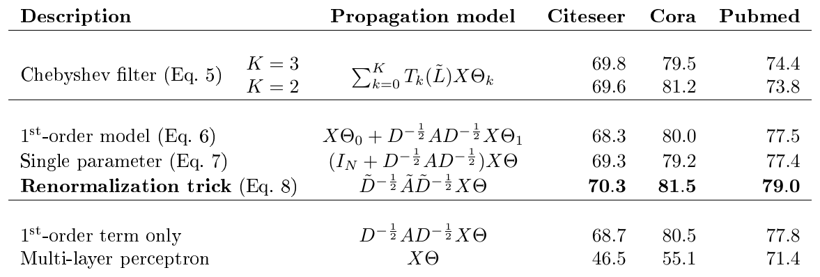
6.2 Evaluation of Propagation Model

We compare different variants of our proposed per-layer propagation model on the citation network datasets. We follow the experimental set-up described in the previous section. Results are summarized in Table 3. The propagation model of our original GCN model is denoted by renormalization trick (in bold). In all other cases, the propagation model of both neural network layers is replaced with the model specified under propagation model. Reported numbers denote mean classification accuracy for 100 repeated runs with random weight matrix initializations. In case of multiple variables $\Theta_i$ per layer, we impose L2 regularization on all weight matrices of the first layer.

6.3 Training Time per Epoch

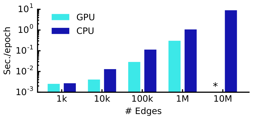
Here, we report results for the mean training time per epoch (forward pass, cross-entropy calculation, backward pass) for 100 epochs on simulated random graphs, measured in seconds wall-clock time. See Section 5.1 for a detailed description of the random graph dataset used in these experiments. We compare results on a GPU and on a CPU-only implementation[^4] in TensorFlow ([12]). Figure 2 summarizes the results.

[^4]: Hardware used: 16-core Intel raise@ Xeon raise@ CPU E5-2640 v3 @ 2.60GHz, GeForce raise@ GTX TITAN X

7. Discussion

Section Summary: The proposed semi-supervised model for node classification achieves stronger accuracy than prior graph-based methods by propagating node features across layers in an end-to-end trainable way, avoiding the restrictive similarity assumptions of Laplacian regularization and the complex multi-stage pipelines of skip-gram approaches. Its renormalized first-order propagation rule further improves both speed and results compared with simpler or higher-order alternatives. The approach still faces practical limits in memory use on very large graphs, support for directed edges or edge attributes, and its fixed assumptions about local neighborhoods, all of which the authors suggest can be addressed through mini-batch training, graph transformations, and learnable trade-off parameters.

7.1 Semi-Supervised Model

In the experiments demonstrated here, our method for semi-supervised node classification outperforms recent related methods by a significant margin. Methods based on graph-Laplacian regularization ([1, 3, 4]) are most likely limited due to their assumption that edges encode mere similarity of nodes. Skip-gram based methods on the other hand are limited by the fact that they are based on a multi-step pipeline which is difficult to optimize. Our proposed model can overcome both limitations, while still comparing favorably in terms of efficiency (measured in wall-clock time) to related methods. Propagation of feature information from neighboring nodes in every layer improves classification performance in comparison to methods like ICA ([29]), where only label information is aggregated.

We have further demonstrated that the proposed renormalized propagation model (Eq.@ Equation 8) offers both improved efficiency (fewer parameters and operations, such as multiplication or addition) and better predictive performance on a number of datasets compared to a naïve $1^{\text{st}}$-order model (Eq.@ Equation 6) or higher-order graph convolutional models using Chebyshev polynomials (Eq.@ Equation 5).

7.2 Limitations and Future Work

Here, we describe several limitations of our current model and outline how these might be overcome in future work.

Memory requirement

In the current setup with full-batch gradient descent, memory requirement grows linearly in the size of the dataset. We have shown that for large graphs that do not fit in GPU memory, training on CPU can still be a viable option. Mini-batch stochastic gradient descent can alleviate this issue. The procedure of generating mini-batches, however, should take into account the number of layers in the GCN model, as the $K^{\text{th}}$-order neighborhood for a GCN with $K$ layers has to be stored in memory for an exact procedure. For very large and densely connected graph datasets, further approximations might be necessary.

Directed edges and edge features

Our framework currently does not naturally support edge features and is limited to undirected graphs (weighted or unweighted). Results on NELL however show that it is possible to handle both directed edges and edge features by representing the original directed graph as an undirected bipartite graph with additional nodes that represent edges in the original graph (see Section 5.1 for details).

Limiting assumptions

Through the approximations introduced in Section 2, we implicitly assume locality (dependence on the $K^{\text{th}}$-order neighborhood for a GCN with $K$ layers) and equal importance of self-connections vs. edges to neighboring nodes. For some datasets, however, it might be beneficial to introduce a trade-off parameter $\lambda$ in the definition of $\tilde{A}$:

$ \tilde{A} = A + \lambda I_N, .\tag{11} $

This parameter now plays a similar role as the trade-off parameter between supervised and unsupervised loss in the typical semi-supervised setting (see Eq.@ Equation 1). Here, however, it can be learned via gradient descent.

8. Conclusion

Section Summary: The authors present a new method for classifying data organized as networks, where only some of the items have known labels. Their GCN model efficiently combines the connections between items with the individual characteristics of each item through a simplified mathematical approximation of graph-based filtering. Tests across several network datasets show that the approach captures useful structure, outperforms recent competing methods, and runs quickly.

We have introduced a novel approach for semi-supervised classification on graph-structured data. Our GCN model uses an efficient layer-wise propagation rule that is based on a first-order approximation of spectral convolutions on graphs. Experiments on a number of network datasets suggest that the proposed GCN model is capable of encoding both graph structure and node features in a way useful for semi-supervised classification. In this setting, our model outperforms several recently proposed methods by a significant margin, while being computationally efficient.

Acknowledgments

We would like to thank Christos Louizos, Taco Cohen, Joan Bruna, Zhilin Yang, Dave Herman, Pramod Sinha and Abdul-Saboor Sheikh for helpful discussions. This research was funded by SAP.

Appendix

Section Summary: The appendix explains how graph convolutional networks relate to the classic Weisfeiler-Lehman algorithm for assigning unique labels to nodes based on graph structure. It shows that the GCN propagation rule can be viewed as a differentiable, trainable version of this algorithm, allowing even an untrained model with random weights to produce useful node embeddings, as demonstrated on the small Zachary karate club network. With minimal semi-supervised training, the model further refines these embeddings to separate communities effectively using only the graph and a few labeled examples.

A. Relation to Weisfeiler-Lehman Algorithm

A neural network model for graph-structured data should ideally be able to learn representations of nodes in a graph, taking both the graph structure and feature description of nodes into account. A well-studied framework for the unique assignment of node labels given a graph and (optionally) discrete initial node labels is provided by the 1-dim Weisfeiler-Lehman (WL-1) algorithm ([7]):

Input: Initial node coloring $(h^{(0)}_1, h^{(0)}_2, ..., h^{(0)}_N )$
Output: Final node coloring $(h^{(T)}_1, h^{(T)}_2, ..., h^{(T)}_N )$
t $\leftarrow$ 0
repeat:
  stable node coloring is reached
untilfor $v_i \in \mathcal{V}$:
  $h^{(t+1)}_i \leftarrow \mathrm{hash}\left(\sum_{j\in\mathcal{N}_i} h^{(t)}_j\right) $
$t \leftarrow t+1$
caption{{WL-1 algorithm citepweisfeiler1968reduction} }

Here, $h_i^{(t)}$ denotes the coloring (label assignment) of node $v_i$ (at iteration $t$) and $\mathcal{N}_i$ is its set of neighboring node indices (irrespective of whether the graph includes self-connections for every node or not). $\mathrm{hash}(\cdot)$ is a hash function. For an in-depth mathematical discussion of the WL-1 algorithm see, e.g., [30].

We can replace the hash function in Algorithm 1 with a neural network layer-like differentiable function with trainable parameters as follows:

$ h^{(l+1)}i = \sigma \left(\sum{j\in\mathcal{N}i} \frac{1}{c{ij}}h^{(l)}_jW^{(l)} \right) , ,\tag{12} $

where $c_{ij}$ is an appropriately chosen normalization constant for the edge $(v_i, v_j)$. Further, we can take $h^{(l)}_i$ now to be a vector of activations of node $i$ in the $l^{\text{th}}$ neural network layer. $W^{(l)}$ is a layer-specific weight matrix and $\sigma(\cdot)$ denotes a differentiable, non-linear activation function.

By choosing $c_{ij}=\sqrt{d_i d_j}$, where $d_i=|\mathcal{N}_i|$ denotes the degree of node $v_i$, we recover the propagation rule of our Graph Convolutional Network (GCN) model in vector form (see Eq.@ Equation 2)[^5].

[^5]: Note that we here implicitly assume that self-connections have already been added to every node in the graph (for a clutter-free notation).

This—loosely speaking—allows us to interpret our GCN model as a differentiable and parameterized generalization of the 1-dim Weisfeiler-Lehman algorithm on graphs.

A.1 Node Embeddings with Random Weights

From the analogy with the Weisfeiler-Lehman algorithm, we can understand that even an untrained GCN model with random weights can serve as a powerful feature extractor for nodes in a graph. As an example, consider the following 3-layer GCN model:

$ Z= \tanh!\left(\hat{A} , \tanh!\left(\hat{A}, \tanh!\left(\hat{A} X W^{(0)}\right) W^{(1)} \right) W^{(2)} \right) , ,\tag{13} $

with weight matrices $W^{(l)}$ initialized at random using the initialization described in [27]. $\hat{A}$, $X$ and $Z$ are defined as in Section 3.1.

We apply this model on Zachary's karate club network ([31]). This graph contains 34 nodes, connected by 154 (undirected and unweighted) edges. Every node is labeled by one of four classes, obtained via modularity-based clustering ([32]). See Figure 3a for an illustration.

We take a featureless approach by setting $X=I_N$, where $I_N$ is the $N$ by $N$ identity matrix. $N$ is the number of nodes in the graph. Note that nodes are randomly ordered (i.e. ordering contains no information). Furthermore, we choose a hidden layer dimensionality[^6] of $4$ and a two-dimensional output (so that the output can immediately be visualized in a 2-dim plot).

[^6]: We originally experimented with a hidden layer dimensionality of $2$ (i.e. same as output layer), but observed that a dimensionality of $4$ resulted in less frequent saturation of $\tanh(\cdot)$ units and therefore visually more pleasing results.

Figure 3b shows a representative example of node embeddings (outputs $Z$) obtained from an untrained GCN model applied to the karate club network. These results are comparable to embeddings obtained from DeepWalk ([14]), which uses a more expensive unsupervised training procedure.

A.2 Semi-Supervised Node Embeddings

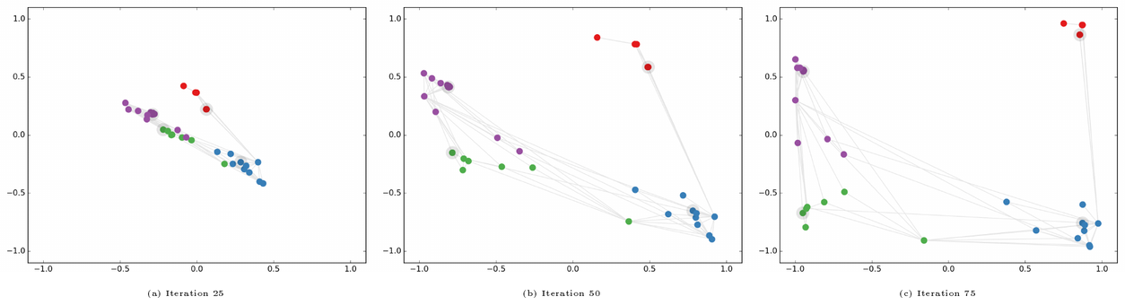
On this simple example of a GCN applied to the karate club network it is interesting to observe how embeddings react during training on a semi-supervised classification task. Such a visualization (see Figure 4) provides insights into how the GCN model can make use of the graph structure (and of features extracted from the graph structure at later layers) to learn embeddings that are useful for a classification task.

We consider the following semi-supervised learning setup: we add a softmax layer on top of our model (Eq.@ Equation 13) and train using only a single labeled example per class (i.e. a total number of 4 labeled nodes). We train for 300 training iterations using Adam ([26]) with a learning rate of $0.01$ on a cross-entropy loss.

Figure 4 shows the evolution of node embeddings over a number of training iterations. The model succeeds in linearly separating the communities based on minimal supervision and the graph structure alone. A video of the full training process can be found on our website^7.

B. Experiments on Model Depth

In these experiments, we investigate the influence of model depth (number of layers) on classification performance. We report results on a 5-fold cross-validation experiment on the Cora, Citeseer and Pubmed datasets ([10]) using all labels. In addition to the standard GCN model (Eq.@ Equation 2), we report results on a model variant where we use residual connections ([8]) between hidden layers to facilitate training of deeper models by enabling the model to carry over information from the previous layer's input:

$ \textstyle H^{(l+1)}= \sigma!\left(\tilde{D}^{-\frac{1}{2}} \tilde{A}\tilde{D}^{-\frac{1}{2}}H^{(l)} W^{(l)} \right) + H^{(l)} , .\tag{14} $

On each cross-validation split, we train for 400 epochs (without early stopping) using the Adam optimizer ([26]) with a learning rate of $0.01$. Other hyperparameters are chosen as follows: 0.5 (dropout rate, first and last layer), $5\cdot 10^{-4}$ (L2 regularization, first layer), 16 (number of units for each hidden layer) and 0.01 (learning rate). Results are summarized in Figure 5.

For the datasets considered here, best results are obtained with a 2- or 3-layer model. We observe that for models deeper than 7 layers, training without the use of residual connections can become difficult, as the effective context size for each node increases by the size of its $K^{\text{th}}$-order neighborhood (for a model with $K$ layers) with each additional layer. Furthermore, overfitting can become an issue as the number of parameters increases with model depth.

References

Section Summary: This section compiles a numbered bibliography of academic papers, books, and software tools that underpin research in graph-based machine learning and semi-supervised learning. The entries span foundational studies on harmonic functions, manifold regularization, and spectral methods from the early 2000s through more recent advances in graph convolutional networks, network embeddings such as DeepWalk and node2vec, and supporting techniques like optimization and visualization. They also include classic references on datasets, graph algorithms, and frameworks such as TensorFlow.

[1] Xiaojin Zhu, Zoubin Ghahramani, and John Lafferty. Semi-supervised learning using gaussian fields and harmonic functions. In International Conference on Machine Learning (ICML), volume 3, pp. 912–919, 2003.

[2] Dengyong Zhou, Olivier Bousquet, Thomas Navin Lal, Jason Weston, and Bernhard Schölkopf. Learning with local and global consistency. In Advances in neural information processing systems (NIPS), volume 16, pp. 321–328, 2004.

[3] Mikhail Belkin, Partha Niyogi, and Vikas Sindhwani. Manifold regularization: A geometric framework for learning from labeled and unlabeled examples. Journal of machine learning research (JMLR), 7(Nov):2399–2434, 2006.

[4] Jason Weston, Frédéric Ratle, Hossein Mobahi, and Ronan Collobert. Deep learning via semi-supervised embedding. In Neural Networks: Tricks of the Trade, pp. 639–655. Springer, 2012.

[5] David K. Hammond, Pierre Vandergheynst, and Rémi Gribonval. Wavelets on graphs via spectral graph theory. Applied and Computational Harmonic Analysis, 30(2):129–150, 2011.

[6] Michaël Defferrard, Xavier Bresson, and Pierre Vandergheynst. Convolutional neural networks on graphs with fast localized spectral filtering. In Advances in neural information processing systems (NIPS), 2016.

[7] Boris Weisfeiler and A. A. Lehmann. A reduction of a graph to a canonical form and an algebra arising during this reduction. Nauchno-Technicheskaya Informatsia, 2(9):12–16, 1968.

[8] Kaiming He, Xiangyu Zhang, Shaoqing Ren, and Jian Sun. Deep residual learning for image recognition. In IEEE Conference on Computer Vision and Pattern Recognition (CVPR), 2016.

[9] Laurens van der Maaten and Geoffrey Hinton. Visualizing data using t-sne. Journal of Machine Learning Research (JMLR), 9(Nov):2579–2605, 2008.

[10] Prithviraj Sen, Galileo Namata, Mustafa Bilgic, Lise Getoor, Brian Galligher, and Tina Eliassi-Rad. Collective classification in network data. AI magazine, 29(3):93, 2008.

[11] Nitish Srivastava, Geoffrey E. Hinton, Alex Krizhevsky, Ilya Sutskever, and Ruslan Salakhutdinov. Dropout: a simple way to prevent neural networks from overfitting. Journal of Machine Learning Research (JMLR), 15(1):1929–1958, 2014.

[12] Mart'ın Abadi et al. TensorFlow: Large-scale machine learning on heterogeneous systems, 2015.

[13] Tomas Mikolov, Ilya Sutskever, Kai Chen, Greg S. Corrado, and Jeff Dean. Distributed representations of words and phrases and their compositionality. In Advances in neural information processing systems (NIPS), pp. 3111–3119, 2013.

[14] Bryan Perozzi, Rami Al-Rfou, and Steven Skiena. Deepwalk: Online learning of social representations. In Proceedings of the 20th ACM SIGKDD international conference on Knowledge discovery and data mining, pp. 701–710. ACM, 2014.

[15] Jian Tang, Meng Qu, Mingzhe Wang, Ming Zhang, Jun Yan, and Qiaozhu Mei. Line: Large-scale information network embedding. In Proceedings of the 24th International Conference on World Wide Web, pp. 1067–1077. ACM, 2015.

[16] Aditya Grover and Jure Leskovec. node2vec: Scalable feature learning for networks. In Proceedings of the 22nd ACM SIGKDD International Conference on Knowledge Discovery and Data Mining. ACM, 2016.

[17] Zhilin Yang, William Cohen, and Ruslan Salakhutdinov. Revisiting semi-supervised learning with graph embeddings. In International Conference on Machine Learning (ICML), 2016.

[18] Marco Gori, Gabriele Monfardini, and Franco Scarselli. A new model for learning in graph domains. In Proceedings. 2005 IEEE International Joint Conference on Neural Networks., volume 2, pp. 729–734. IEEE, 2005.

[19] Franco Scarselli, Marco Gori, Ah Chung Tsoi, Markus Hagenbuchner, and Gabriele Monfardini. The graph neural network model. IEEE Transactions on Neural Networks, 20(1):61–80, 2009.

[20] Yujia Li, Daniel Tarlow, Marc Brockschmidt, and Richard Zemel. Gated graph sequence neural networks. In International Conference on Learning Representations (ICLR), 2016.

[21] David K. Duvenaud, Dougal Maclaurin, Jorge Iparraguirre, Rafael Bombarell, Timothy Hirzel, Alán Aspuru-Guzik, and Ryan P. Adams. Convolutional networks on graphs for learning molecular fingerprints. In Advances in neural information processing systems (NIPS), pp. 2224–2232, 2015.

[22] James Atwood and Don Towsley. Diffusion-convolutional neural networks. In Advances in neural information processing systems (NIPS), 2016.

[23] Mathias Niepert, Mohamed Ahmed, and Konstantin Kutzkov. Learning convolutional neural networks for graphs. In International Conference on Machine Learning (ICML), 2016.

[24] Joan Bruna, Wojciech Zaremba, Arthur Szlam, and Yann LeCun. Spectral networks and locally connected networks on graphs. In International Conference on Learning Representations (ICLR), 2014.

[25] Andrew Carlson, Justin Betteridge, Bryan Kisiel, Burr Settles, Estevam R. Hruschka Jr, and Tom M. Mitchell. Toward an architecture for never-ending language learning. In AAAI, volume 5, pp. 3, 2010.

[26] Diederik P. Kingma and Jimmy Lei Ba. Adam: A method for stochastic optimization. In International Conference on Learning Representations (ICLR), 2015.

[27] Xavier Glorot and Yoshua Bengio. Understanding the difficulty of training deep feedforward neural networks. In AISTATS, volume 9, pp. 249–256, 2010.

[28] Thorsten Joachims. Transductive inference for text classification using support vector machines. In International Conference on Machine Learning (ICML), volume 99, pp. 200–209, 1999.

[29] Qing Lu and Lise Getoor. Link-based classification. In International Conference on Machine Learning (ICML), volume 3, pp. 496–503, 2003.

[30] Brendan L. Douglas. The Weisfeiler-Lehman method and graph isomorphism testing. arXiv preprint arXiv:1101.5211, 2011.

[31] Wayne W. Zachary. An information flow model for conflict and fission in small groups. Journal of anthropological research, pp. 452–473, 1977.

[32] Ulrik Brandes, Daniel Delling, Marco Gaertler, Robert Gorke, Martin Hoefer, Zoran Nikoloski, and Dorothea Wagner. On modularity clustering. IEEE Transactions on Knowledge and Data Engineering, 20(2):172–188, 2008.