VAE with a VampPrior

Jakub M. Tomczak
University of Amsterdam

Max Welling
University of Amsterdam

Abstract

Many different methods to train deep generative models have been introduced in the past. In this paper, we propose to extend the variational auto-encoder (VAE) framework with a new type of prior which we call "Variational Mixture of Posteriors" prior, or VampPrior for short. The VampPrior consists of a mixture distribution (e.g., a mixture of Gaussians) with components given by variational posteriors conditioned on learnable pseudo-inputs. We further extend this prior to a two layer hierarchical model and show that this architecture with a coupled prior and posterior, learns significantly better models. The model also avoids the usual local optima issues related to useless latent dimensions that plague VAEs. We provide empirical studies on six datasets, namely, static and binary MNIST, OMNIGLOT, Caltech 101 Silhouettes, Frey Faces and Histopathology patches, and show that applying the hierarchical VampPrior delivers state-of-the-art results on all datasets in the unsupervised permutation invariant setting and the best results or comparable to SOTA methods for the approach with convolutional networks.

Executive Summary: This paper addresses a key challenge in machine learning: building generative models that can accurately capture complex patterns in large datasets, such as image collections, to enable tasks like data synthesis, anomaly detection, and representation learning. Traditional variational auto-encoders (VAEs), a popular framework for this, often underperform because they use a simple prior distribution—typically a standard normal—that overly constrains the model's hidden representations, leading to poor fits and underused latent variables. This issue is pressing now as deep learning applications expand into areas like medical imaging and creative AI, where high-fidelity models are essential for reliable outcomes.

The work aims to improve VAEs by introducing a more flexible prior called the Variational Mixture of Posteriors (VampPrior), which approximates an optimal data-driven prior using a mixture of encoder distributions conditioned on learnable "pseudo-inputs." It also extends this to a two-layer hierarchical VAE to better handle deep structures and unused latent dimensions.

The authors derived the VampPrior theoretically by reformulating the VAE's objective to emphasize matching the prior to the average data posterior while avoiding overfitting through a limited number of pseudo-inputs (e.g., 500 per dataset). They tested it empirically on six image datasets—static and dynamic handwritten digits (MNIST), characters (Omniglot), object silhouettes (Caltech 101), faces (Frey Faces), and medical patches (Histopathology)—spanning 2,000 to 60,000 training images from 2011–2016 sources. Models used neural networks with 40 latent units per layer, trained via stochastic optimization over 100+ epochs; comparisons included standard priors, mixture-of-Gaussians alternatives, and state-of-the-art methods, with performance measured by log-likelihood on held-out test sets.

Key results show the VampPrior consistently boosted generative performance over the standard normal prior, improving average test log-likelihood by 2–9 units (e.g., from -88.6 to -85.6 on static MNIST, equivalent to better data density estimates). The hierarchical VampPrior VAE achieved top or near-top results across all datasets in a basic neural network setup, outperforming prior benchmarks by 1–20 units where applicable (e.g., -83.2 on static MNIST vs. -85.1 for enhanced VAEs). It activated 1.5–4 times more latent units than standard hierarchical VAEs, reducing wasted dimensions. With convolutional networks, gains narrowed the gap to advanced models, reaching state-of-the-art on dynamic MNIST (-78.5) and Omniglot (-89.8). Qualitatively, generated and reconstructed images were sharper and more detailed, with pseudo-inputs forming interpretable prototypes like digit shapes.

These findings mean VAEs can now learn richer, more efficient hidden representations without over-regularization, enhancing model utility for downstream tasks like image synthesis or classification pre-training. Unlike expectations of simple priors sufficing, the VampPrior's coupling with the encoder promotes high-variance mappings that better reflect data diversity, cutting risks of mode collapse and improving output quality—potentially lowering costs in data-scarce fields like healthcare by generating realistic samples. This outperforms uncoupled alternatives like mixture-of-Gaussians priors by 1–3 units, highlighting the value of trainable integration.

Decision-makers should integrate the VampPrior into VAE pipelines for image-based applications, starting with the hierarchical version to maximize latent efficiency; for speed-critical uses, pair it with convolutional decoders despite a 1.4–2x training time increase. Trade-offs include slightly higher compute vs. superior fits (e.g., worth it for accuracy gains >5%). Further pilots are recommended: test on non-image data like text or audio, and combine with techniques like normalizing flows or adversarial training to push performance further before full deployment.

While robust across datasets, limitations include reliance on Gaussian assumptions for latents (potentially missing multimodal data traits) and added complexity from pseudo-inputs, which can noise up in small datasets like Frey Faces. Confidence is high in the improvements for image generation, backed by consistent quantitative and visual evidence, but caution is advised for extrapolation to sequential data without validation.

1. Introduction

Section Summary: Learning generative models that can create complex patterns from huge datasets, like collections of images, is a big challenge in machine learning, and variational auto-encoders (VAEs) have emerged as an efficient way to tackle this using techniques like the reparameterization trick. However, simple priors, such as the standard normal distribution, often cause over-regularization and weak hidden representations, so this paper examines the regularization in VAEs' training objective and proposes a new "VampPrior"—a flexible mixture of variational posteriors based on learnable pseudo-data—to make the model more powerful. The authors also introduce a two-level VAE architecture using this prior, which avoids wasted latent dimensions and empirically outperforms standard approaches on six datasets, achieving top results.

Learning generative models that are capable of capturing rich distributions from vast amounts of data like image collections remains one of the major challenges of machine learning. In recent years, different approaches to achieving this goal were proposed by formulating alternative training objectives to the log-likelihood [1, 2, 3] or by utilizing variational inference [4]. The latter approach could be made especially efficient through the application of the reparameterization trick resulting in a highly scalable framework now known as the variational auto-encoders (VAE) [5, 6]. Various extensions to deep generative models have been proposed that aim to enrich the variational posterior [7, 8, 9, 10, 11, 12]. Recently, it has been noticed that in fact the prior plays a crucial role in mediating between the generative decoder and the variational encoder. Choosing a too simplistic prior like the standard normal distribution could lead to over-regularization and, as a consequence, very poor hidden representations [13].

In this paper, we take a closer look at the regularization term of the variational lower bound inspired by the analysis presented in [14]. Re-formulating the variational lower bound gives two regularization terms: the average entropy of the variational posterior, and the cross-entropy between the averaged (over the training data) variational posterior and the prior. The cross-entropy term can be minimized by setting the prior equal to the average of the variational posteriors over training points. However, this would be computationally very expensive. Instead, we propose a new prior that is a variational mixture of posteriors prior, or VampPrior for short. Moreover, we present a new two-level VAE that combined with our new prior can learn a very powerful hidden representation.

The contribution of the paper is threefold:

• We follow the line of research of improving the VAE by making the prior more flexible. We propose a new prior that is a mixture of variational posteriors conditioned on learnable pseudo-data. This allows the variational posterior to learn more a potent latent representation.
• We propose a new two-layered generative VAE model with two layers of stochastic latent variables based on the VampPrior idea. This architecture effectively avoids the problems of unused latent dimensions.
• We show empirically that the VampPrior always outperforms the standard normal prior in different VAE architectures and that the hierarchical VampPrior based VAE achieves state-of-the-art or comparable to SOTA results on six datasets.

2. Variational Auto-Encoder

Let $\mathbf{x}$ be a vector of $D$ observable variables and $\mathbf{z} \in \mathbb{R}^{M}$ a vector of stochastic latent variables. Further, let $p_{\theta}(\mathbf{x}, \mathbf{z})$ be a parametric model of the joint distribution. Given data $\mathbf{X} = {\mathbf{x}1, \ldots, \mathbf{x}N}$ we typically aim at maximizing the average marginal log-likelihood, $\frac{1}{N} \ln p(\mathbf{X}) = \frac{1}{N}\sum{i=1}^{N} \ln p(\mathbf{x}{i})$, with respect to parameters. However, when the model is parameterized by a neural network (NN), the optimization could be difficult due to the intractability of the marginal likelihood. One possible way of overcoming this issue is to apply variational inference and optimize the following lower bound:

$ \begin{align} \mathbb{E}{\mathbf{x} \sim q(\mathbf{x})}[\ln p(\mathbf{x})] \geq& \mathbb{E}{\mathbf{x} \sim q(\mathbf{x})} \big[\mathbb{E}{q{\phi}(\mathbf{z}|\mathbf{x})}[\ln p_{\theta}(\mathbf{x}|\mathbf{z}) + \nonumber \ &+ \ln p_{\lambda}(\mathbf{z}) - \ln q_{\phi}(\mathbf{z}|\mathbf{x})] \big] \ \stackrel{\Delta}{=}& \mathcal{L}(\phi, \theta, \lambda), \nonumber \end{align}\tag{1} $

where $q(\mathbf{x}) = \frac{1}{N} \sum_{n=1}^{N} \delta(\mathbf{x} - \mathbf{x}{n})$ is the empirical distribution, $q{\phi}(\mathbf{z}|\mathbf{x})$ is the variational posterior (the encoder), $p_{\theta}(\mathbf{x}|\mathbf{z})$ is the generative model (the decoder) and $p_{\lambda}(\mathbf{z})$ is the prior, and $\phi, \theta, \lambda$ are their parameters, respectively.

There are various ways of optimizing this lower bound but for continuous $\mathbf{z}$ this could be done efficiently through the re-parameterization of $q_{\phi}(\mathbf{z}|\mathbf{x})$ [5, 6], which yields a variational auto-encoder architecture (VAE). Therefore, during learning we consider a Monte Carlo estimate of the second expectation in Equation (1) using $L$ sample points:

$ \begin{align} \widetilde{ \mathcal{L} }(\phi, \theta, \lambda) =& \mathbb{E}{\mathbf{x} \sim q(\mathbf{x})} \Big[\frac{1}{L} \sum{l=1}^{L} \big(\ln p_{\theta}(\mathbf{x}|\mathbf{z}{\phi}^{(l)}) + \tag{a} \ &+ \ln p{\lambda}(\mathbf{z}{\phi}^{(l)}) - \ln q{\phi}(\mathbf{z}_{\phi}^{(l)}|\mathbf{x}) \big) \Big], \tag{b} \end{align}\tag{2} $

where $\mathbf{z}{\phi}^{(l)}$ are sampled from $q\phi(\mathbf{z}|\mathbf{x})$ through the re-parameterization trick.

The first component of the objective function can be seen as the expectation of the negative reconstruction error that forces the hidden representation for each data case to be peaked at its specific MAP value. On the contrary, the second and third components constitute a kind of regularization that drives the encoder to match the prior.

We can get more insight into the role of the prior by inspecting the gradient of $\widetilde{ \mathcal{L} }(\phi, \theta, \lambda)$ in Equation (2a) and (2b) with respect to a single weight $\phi_{i}$ for a single data point $\mathbf{x}$, see Eq. (7a) and (7b) in Supplementary Material for details. We notice that the prior plays a role of an ''anchor'' that keeps the posterior close to it, i.e., the term in round brackets in Eq. (7b) is $0$ if the posterior matches the prior.

Typically, the encoder is assumed to have a diagonal covariance matrix, i.e., $q_{\phi}(\mathbf{z}|\mathbf{x}) = \mathcal{N}\big(\mathbf{z}|\mu_{\phi}(\mathbf{x}), \mathrm{diag}(\sigma_{\phi}^{2}(\mathbf{x})) \big)$, where $\mu_{\phi}(\mathbf{x})$ and $\sigma_{\phi}^{2}(\mathbf{x})$ are parameterized by a NN with weights $\phi$, and the prior is expressed using the standard normal distribution, $p_{\lambda}(\mathbf{z}) = \mathcal{N}(\mathbf{z} | \mathbf{0}, \mathbf{I})$. The decoder utilizes a suitable distribution for the data under consideration, e.g., the Bernoulli distribution for binary data or the normal distribution for continuous data, and it is parameterized by a NN with weights $\theta$.

3. The Variational Mixture of Posteriors Prior

Section Summary: In variational autoencoders, the standard prior like a normal distribution often over-regularizes the model, limiting its latent dimensions. To address this, researchers rewrite the training objective to better align the prior with the data's aggregated posterior, but directly using that aggregated posterior risks overfitting and high computation, so they approximate it with a variational mixture of posteriors based on learned pseudo-inputs, called the VampPrior. This multimodal prior promotes higher variability in the model's hidden representations while keeping training efficient, outperforming simpler alternatives like mixtures of Gaussians by fostering better coordination between the prior and the encoder during learning.

Idea

The variational lower-bound consists of two parts, namely, the reconstruction error and the regularization term between the encoder and the prior. However, we can re-write the training objective Equation (1) to obtain two regularization terms instead of one [14]:

$ \begin{align} \mathcal{L}(\phi, \theta, \lambda) =& \mathbb{E}{\mathbf{x} \sim q(\mathbf{x})} \big[\mathbb{E}{q_{\phi}(\mathbf{z}|\mathbf{x})}[\ln p_{\theta}(\mathbf{x}|\mathbf{z})] \big] + \ &+ \mathbb{E}{\mathbf{x} \sim q(\mathbf{x})} \big[\mathbb{H}[q{\phi}(\mathbf{z}|\mathbf{x})] \big] + \ &- \mathbb{E}{\mathbf{z} \sim q(\mathbf{z}) } [-\ln p{\lambda}(\mathbf{z})] \end{align}\tag{3} $

where the first component is the negative reconstruction error, the second component is the expectation of the entropy $\mathbb{H}[\cdot]$ of the variational posterior and the last component is the cross-entropy between the aggregated posterior [13, 14], $q(\mathbf{z}) = \frac{1}{N} \sum_{n=1}^{N} q_{\phi}(\mathbf{z}|\mathbf{x}_{n})$, and the prior. The second term of the objective encourages the encoder to have large entropy (e.g., high variance) for every data case. The last term aims at matching the aggregated posterior and the prior.

Usually, the prior is chosen in advance, e.g., a standard normal prior. However, one could find a prior that optimizes the ELBO by maximizing the following Lagrange function with the Lagrange multiplier $\beta$:

$ \max_{p_{\lambda}(\mathbf{z})} - \mathbb{E}{\mathbf{z} \sim q(\mathbf{z}) } [-\ln p{\lambda}(\mathbf{z})] + \beta \Big(\int p_{\lambda}(\mathbf{z}) \mathrm{d} \mathbf{z} - 1 \Big).\tag{4} $

The solution of this problem is simply the aggregated posterior:

$ p_{\lambda}^{*}(\mathbf{z}) = \frac{1}{N} \sum_{n=1}^{N} q_{\phi}(\mathbf{z}|\mathbf{x}_{n}). $

However, this choice may potentially lead to overfitting [13, 14] and definitely optimizing the recognition model would become very expensive due to the sum over all training points. On the other hand, having a simple prior like the standard normal distribution is known to result in over-regularized models with only few active latent dimensions [15].

In order to overcome issues like overfitting, over-regularization and high computational complexity, the optimal solution, i.e., the aggregated posterior, can be further approximated by a mixture of variational posteriors with pseudo-inputs:

$ p_{\lambda}(\mathbf{z}) = \frac{1}{K} \sum_{k=1}^{K} q_{\phi}(\mathbf{z}|\mathbf{u}_{k}), $

where $K$ is the number of pseudo-inputs, and $\mathbf{u}{k}$ is a $D$-dimensional vector we refer to as a pseudo-input. The pseudo-inputs are learned through backpropagation and can be thought of as hyperparameters of the prior, alongside parameters of the posterior $\phi$, $\lambda = {\mathbf{u}{1}, \ldots, \mathbf{u}_{K}, \phi}$. Importantly, the resulting prior is multimodal, thus, it prevents the variational posterior to be over-regularized. On the other hand, incorporating pseudo-inputs prevents from potential overfitting once we pick $K \ll N$, which also makes the model less expensive to train. We refer to this prior as the variational mixture of posteriors prior (VampPrior).

A comparison to a mixture of Gaussians prior

A simpler alternative to the VampPrior that still approximates the optimal solution of the problem in Equation (4) is a mixture of Gaussians (MoG), $p_{\lambda}(\mathbf{z}) = \frac{1}{K} \sum_{k=1}^{K} \mathcal{N} \big(\mu_k, \mathrm{diag}(\sigma_{k}^{2}) \big)$. The hyperparameters of the prior $\lambda = {\mu_{k}, \mathrm{diag}(\sigma_{k}^{2}) }_{k=1}^{K}$ are trained by backpropagation similarly to the pseudo-inputs. The MoG prior influences the variational posterior in the same manner to the standard prior and the gradient of the ELBO with respect to the encoder's parameters takes an analogous form to (7a) and (7b), see Suplementary Material for details.

In the case of the VampPrior, on the other hand, we obtain two advantages over the MoG prior:

• First, by coupling the prior with the posterior we entertain fewer parameters and the prior and variational posteriors will at all times "cooperate" during training.
• Second, this coupling highly influences the gradient wrt a single weight of the encoder, $\phi_{i}$, for a given $\mathbf{x}$, see Eq. (8a b) and (8a c) in Supplementary Material for details. The differences in Equation (8a b) and (8a c) are close to $0$ as long as $q_{\phi}(\mathbf{z}{\phi}^{(l)} | \mathbf{x}) \approx q{\phi}(\mathbf{z}{\phi}^{(l)} | \mathbf{u}{k})$. Thus, the gradient is influenced by pseudo-inputs that are dissimilar to $\mathbf{x}$, i.e., if the posterior produces different hidden representations for $\mathbf{u}_{k}$ and $\mathbf{x}$. In other words, since this has to hold for every training case, the gradient points towards a solution where the variational posterior has high variance. On the contrary, the first part of the objective in Equation (8a a) causes the posteriors to have low variance and map to different latent explanations for each data case. These effects distinguish the VampPrior from the MoG prior utilized in the VAE so far [16, 8].

A connection to the Empirical Bayes

The idea of the Empirical Bayes (EB), also known as the type-II maximum likelihood, is to find hyperparameters $\lambda$ of the prior over latent variables $\mathbf{z}$, $p(\mathbf{z}|\lambda)$, by maximizing the marginal likelihood $p(\mathbf{x}|\lambda)$. In the case of the VAE and the VampPrior the pseudo-inputs, alongside the parameters of the posterior, are the hyperparameters of the prior and we aim at maximizing the ELBO with respect to them. Thus, our approach is closely related to the EB and in fact it formulates a new kind of Bayesian inference that combines the variational inference with the EB approach.

A connection to the Information Bottleneck

We have shown that the aggregated posterior is the optimal prior within the VAE formulation. This result is closely related to the Information Bottleneck (IB) approach [17, 18] where the aggregated posterior naturally plays the role of the prior. Interestingly, the VampPrior brings the VAE and the IB formulations together and highlights their close relation. A similar conclusion and a more thorough analysis of the close relation between the VAE and the IB through the VampPrior is presented in [19].

4. Hierarchical VampPrior Variational Auto-Encoder

Section Summary: A common issue in training variational auto-encoders (VAEs) is that some hidden units become inactive, especially in deeper models where layers farther from the data struggle to learn useful patterns. To fix this, the authors introduce a two-layer hierarchical VAE that uses a rich, VampPrior distribution for the base layer, helping the model generate and infer data more effectively across layers with neural networks parameterizing the key distributions. They also test simpler alternatives like a standard Gaussian prior, a fixed mixture of Gaussians, and a VampPrior version using real data samples to see if complexity is truly needed for better performance.

Hierarchical VAE and the inactive stochastic latent variable problem

A typical problem encountered during training a VAE is the inactive stochastic units [15, 20]. Our VampPrior VAE seems to be an effective remedy against this issue, simply because the prior is designed to be rich and multimodal, preventing the KL term from pulling individual posteriors towards a simple (e.g., standard normal) prior. The inactive stochastic units problem is even worse for learning deeper VAEs (i.e., with multiple layers of stochastic units). The reason might be that stochastic dependencies within a deep generative model are top-down in the generative process and bottom-up in the variational process. As a result, there is less information obtained from real data at the deeper stochastic layers, making them more prone to become regularized towards the prior.

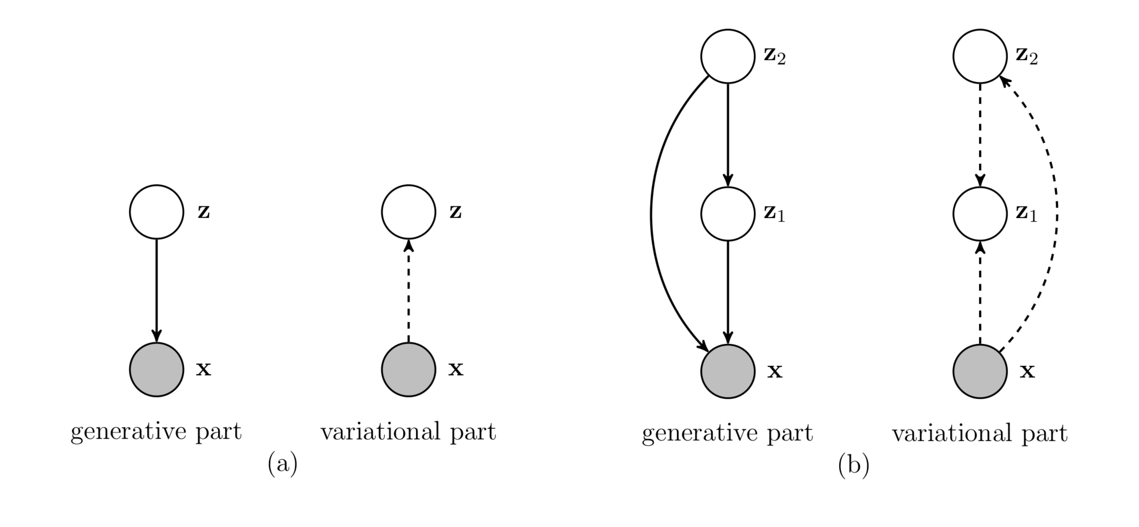
In order to prevent a deep generative model to suffer from the inactive stochastic units problem we propose a new two-layered VAE as follows:

$ q_{\phi}(\mathbf{z}1 | \mathbf{x}, \mathbf{z}{2})\ q_{\psi}(\mathbf{z}_{2} | \mathbf{x}),\tag{5} $

while the the generative part is the following:

$ p_{\theta}(\mathbf{x} | \mathbf{z}{1}, \mathbf{z}{2})\ p_{\lambda}(\mathbf{z}1 | \mathbf{z}{2})\ p(\mathbf{z}_{2}),\tag{6} $

with $p(\mathbf{z}_{2})$ given by a VampPrior. The model is depicted in Figure 1(b).

In this model we use normal distributions with diagonal covariance matrices to model $\mathbf{z}_1 \in \mathbb{R}^{M_1}$ and $\mathbf{z}_2 \in \mathbb{R}^{M_2}$, parameterized by NNs. The full model is given by:

$ \begin{align} p(\mathbf{z}{2}) &= \frac{1}{K} \sum{k=1}^{K} q_{\psi}(\mathbf{z}{2} | \mathbf{u}{k}), \ p_{\lambda}(\mathbf{z}1 | \mathbf{z}{2}) &= \mathcal{N}\big(\mathbf{z}1|\mu{\lambda}(\mathbf{z}2), \mathrm{diag}(\sigma{\lambda}^{2}(\mathbf{z}2)) \big), \ q{\phi}(\mathbf{z}1 | \mathbf{x}, \mathbf{z}{2}) &= \mathcal{N}\big(\mathbf{z}1|\mu{\phi}(\mathbf{x}, \mathbf{z}{2}), \mathrm{diag}(\sigma{\phi}^{2}(\mathbf{x}, \mathbf{z}{2})) \big), \ q{\psi}(\mathbf{z}2 | \mathbf{x}) &= \mathcal{N}\big(\mathbf{z}2|\mu{\psi}(\mathbf{x}), \mathrm{diag}(\sigma{\psi}^{2}(\mathbf{x})) \big) . \end{align} $

Alternative priors

We have motivated the VampPrior by analyzing the variational lower bound. However, one could inquire whether we really need such complicated prior and maybe the proposed two-layered VAE is already sufficiently powerful. In order to answer these questions we further verify three alternative priors:

• the standard Gaussian prior (SG):

$ p(\mathbf{z}_{2}) = \mathcal{N}(\mathbf{0}, \mathbf{I}); $

• the mixture of Gaussians prior (MoG):

$ p(\mathbf{z}{2}) = \frac{1}{K} \sum{k=1}^{K} \mathcal{N} \big(\mu_k, \mathrm{diag}(\sigma_{k}^{2}) \big), $

where $\mu_{k} \in \mathbb{R}^{M_2}$, $\sigma_{k}^{2} \in \mathbb{R}^{M_2}$ are trainable parameters;

• the VampPrior with a random subset of real training data as non-trainable pseudo-inputs (VampPrior data).

Including the standard prior can provide us with an answer to the general question if there is even a need for complex priors. Utilizing the mixture of Gaussians verifies whether it is beneficial to couple the prior with the variational posterior or not. Finally, using a subset of real training images determines to what extent it is useful to introduce trainable pseudo-inputs.

5. Experiments

Section Summary: The experiments test whether a technique called VampPrior improves how variational autoencoders (VAEs) learn patterns in image data and whether a two-layer generative model outperforms simpler single-layer versions. Researchers compared various setups using basic or advanced neural networks on six image datasets, training them with standard methods and evaluating performance through likelihood scores that measure how well models capture data variations. Overall, models with VampPrior achieved higher scores than those with standard priors, and the new hierarchical approach matched or exceeded many leading techniques on key benchmarks.

5.1 Setup

In the experiments we aim at: (i) verifying empirically whether the VampPrior helps the VAE to train a representation that better reflects variations in data, and (ii) inspecting if our proposition of a two-level generative model performs better than the one-layered model. In order to answer these questions we compare different models parameterized by feed-forward neural networks (MLPs) or convolutional networks that utilize the standard prior and the VampPrior. In order to compare the hierarchical VampPrior VAE with the state-of-the-art approaches, we used also an autoregressive decoder. Nevertheless, our primary goal is to quantitatively and qualitatively assess the newly proposed prior.

We carry out experiments using six image datasets: static MNIST [21], dynamic MNIST [22], OMNIGLOT [23], Caltech 101 Silhouette [24], Frey Faces^1 and Histopathology patches [11]. More details about the datasets can be found in the Supplementary Material.

In the experiments we modeled all distributions using MLPs with two hidden layers of $300$ hidden units in the unsupervised permutation invariant setting. We utilized the gating mechanism as an element-wise non-linearity [25]. We utilized $40$ stochastic hidden units for both $\mathbf{z}_1$ and $\mathbf{z}_2$. Next we replaced MLPs with convolutional layers with gating mechanism. Eventually, we verified also a PixelCNN [26] as the decoder. For Frey Faces and Histopathology we used the discretized logistic distribution of images as in [27], and for other datasets we applied the Bernoulli distribution.

For learning the ADAM algorithm [28] with normalized gradients [29] was utilized with the learning rate in ${10^{-4}, 5\cdot 10^{-4}}$ and mini-batches of size $100$. Additionally, to boost the generative capabilities of the decoder, we used the warm-up for $100$ epochs [30]. The weights of the neural networks were initialized according to [31]. The early-stopping with a look ahead of $50$ iterations was applied. For the VampPrior we used $500$ pseudo-inputs for all datasets except OMNIGLOT for which we utilized $1000$ pseudo-inputs. For the VampPrior data we randomly picked training images instead of the learnable pseudo-inputs.

We denote the hierarchical VAE proposed in this paper with MLPs by $\textsc{HVAE}$, while the hierarchical VAE with convolutional layers and additionally with a PixelCNN decoder are denoted by $\textsc{convHVAE}$ and $\textsc{PixelHVAE}$, respectively.

5.2 Results

\begin{tabular}{c|cc|cc|cc|cc|cc}
 & \multicolumn{2}{c|}{\footnotesize{\textsc{VAE} ($L=1$)}} & \multicolumn{2}{c|}{\footnotesize{\textsc{HVAE} ($L=2$)}} & \multicolumn{2}{c|}{\footnotesize{\textsc{convHVAE} ($L=2$)}} & \multicolumn{2}{c|}{\footnotesize{\textsc{PixelHVAE} ($L=2$)}}\\
\textsc{Dataset} & {\fontsize{7}{8.4}\selectfont standard} & {\fontsize{7}{8.4}\selectfont VampPrior} & {\fontsize{7}{8.4}\selectfont standard} & {\fontsize{7}{8.4}\selectfont VampPrior} & {\fontsize{7}{8.4}\selectfont standard} & {\fontsize{7}{8.4}\selectfont VampPrior} & {\fontsize{7}{8.4}\selectfont standard} & {\fontsize{7}{8.4}\selectfont VampPrior} \\
\hline
{\fontsize{7}{8.4}\selectfont staticMNIST } & $-88.56$ & $\mathbf{-85.57}$ & $-86.05$ & $\mathbf{-83.19}$ & $-82.41$ & $\mathbf{-81.09}$ & $-80.58$ & $\mathbf{-79.78}$ \\
{\fontsize{7}{8.4}\selectfont dynamicMNIST } & $-84.50$ & $\mathbf{-82.38}$ & $-82.42$ & $\mathbf{-81.24}$ & $-80.40$ & $\mathbf{-79.75}$ & $-79.70$ & $\mathbf{-78.45}$ \\
{\fontsize{7}{8.4}\selectfont Omniglot } & $-108.50$ & $\mathbf{-104.75}$ & $-103.52$ & $\mathbf{-101.18}$ & $-97.65$ & $\mathbf{-97.56}$ & $-90.11$ & $\mathbf{-89.76}$ \\
{\fontsize{7}{8.4}\selectfont Caltech 101} & $-123.43$ & $\mathbf{-114.55}$ & $-112.08$ & $\mathbf{-108.28}$ & $-106.35$ & $\mathbf{-104.22}$ & $\mathbf{-85.51}$ & $-86.22$ \\
{\fontsize{7}{8.4}\selectfont Frey Faces } & $4.63$ & $\mathbf{4.57}$ & $4.61$ & $\mathbf{4.51}$ & $4.49$ & $\mathbf{4.45}$ & $4.43$ & $\mathbf{4.38}$ \\
{\fontsize{7}{8.4}\selectfont Histopathology } & $6.07$ & $\mathbf{6.04}$ & $5.82$ & $\mathbf{5.75}$ & $5.59$ & $\mathbf{5.58}$ & $4.84$ & $\mathbf{4.82}$ 
\end{tabular}

Quantitative results

We quantitatively evaluate our method using the test marginal log-likelihood (LL) estimated using the Importance Sampling with 5, 000 sample points [15, 6]. In Table 1 we present a comparison between models with the standard prior and the VampPrior. The results of our approach in comparison to the state-of-the-art methods are gathered in Table 2, Table 3, Table 4 and Table 5 for static and dynamic MNIST, OMNIGLOT and Caltech 101 Silhouettes, respectively.

:Table 2: Test LL for static MNIST.

$\textsc{Model}$	$\textsc{LL}$
$\textsc{VAE (L=1) + NF}$ [9]	$-85.10$
$\textsc{VAE (L=2)}$ [15]	$-87.86$
$\textsc{IWAE (L=2)}$ [15]	$-85.32$
$\textsc{HVAE (L=2) + SG}$	$-85.89$
$\textsc{HVAE (L=2) + MoG}$	$-85.07$
$\textsc{HVAE (L=2) + VampPrior}$ data	$-85.71$
$\textsc{HVAE (L=2) + VampPrior}$	$\mathbf{-83.19}$
$\textsc{AVB + AC (L=1)}$ [32]	$-80.20$
$\textsc{VLAE}$ [33]	$\mathbf{-79.03}$
$\textsc{VAE + IAF}$ [27]	$-79.88$
$\textsc{convHVAE (L=2) + VampPrior}$	$-81.09$
$\textsc{PixelHVAE (L=2) + VampPrior}$	$-79.78$

:Table 3: Test LL for dynamic MNIST.

$\textsc{Model}$	$\textsc{LL}$
$\textsc{VAE (L=2) + VGP}$ [12]	$-81.32$
$\textsc{CaGeM-0 (L=2) [20]}$	$-81.60$
$\textsc{LVAE (L=5) [34]}$	$-81.74$
$\textsc{HVAE (L=2) + VampPrior}$ data	$-81.71$
$\textsc{HVAE (L=2) + VampPrior}$	$\mathbf{-81.24}$
$\textsc{VLAE}$ [33]	$-78.53$
$\textsc{VAE + IAF}$ [27]	$-79.10$
$\textsc{PixelVAE}$ [35]	$-78.96$
$\textsc{convHVAE (L=2) + VampPrior}$	$-79.78$
$\textsc{PixelHVAE (L=2) + VampPrior}$	$\mathbf{-78.45}$

:Table 4: Test LL for OMNIGLOT.

$\textsc{Model}$	$\textsc{LL}$
$\textsc{VR-max (L=2)}$ [36]	$-103.72$
$\textsc{IWAE (L=2)}$ [15]	$-103.38$
$\textsc{LVAE (L=5)}$ [34]	$-102.11$
$\textsc{HVAE (L=2) + VampPrior}$	$\mathbf{-101.18}$
$\textsc{VLAE}$ [33]	$-89.83$
$\textsc{convHVAE (L=2) + VampPrior}$	$-97.56$
$\textsc{PixelHVAE (L=2) + VampPrior}$	$\mathbf{-89.76}$

:Table 5: Test LL for Caltech 101 Silhouettes.

$\textsc{Model}$	$\textsc{LL}$
$\textsc{IWAE (L=1)}$ [36]	$-117.21$
$\textsc{VR-max (L=1)}$ [36]	$-117.10$
$\textsc{HVAE (L=2) + VampPrior}$	$\mathbf{-108.28}$
$\textsc{VLAE}$ [33]	$\mathbf{-78.53}$
$\textsc{convHVAE (L=2) + VampPrior}$	$-104.22$
$\textsc{PixelHVAE (L=2) + VampPrior}$	$-86.22$

First we notice that in all cases except one the application of the VampPrior results in a substantial improvement of the generative performance in terms of the test LL comparing to the standard normal prior (see Table 1). This confirms our supposition that a combination of multimodality and coupling the prior with the posterior is superior to the standard normal prior. Further, we want to stress out that the VampPrior outperforms other priors like a single Gaussian or a mixture of Gaussians (see Table 2). These results provide an additional evidence that the VampPrior leads to a more powerful latent representation and it differs from the MoG prior. We also examined whether the presented two-layered model performs better than the widely used hierarchical architecture of the VAE. Indeed, the newly proposed approach is more powerful even with the SG prior (HVAE ($L=2$) + SG) than the standard two-layered VAE (see Table 2). Applying the MoG prior results in an additional boost of performance. This provides evidence for the usefulness of a multimodal prior. The VampPrior data gives only slight improvement comparing to the SG prior and because of the application of the fixed training data as the pseudo-inputs it is less flexible than the MoG. Eventually, coupling the variational posterior with the prior and introducing learnable pseudo-inputs gives the best performance.

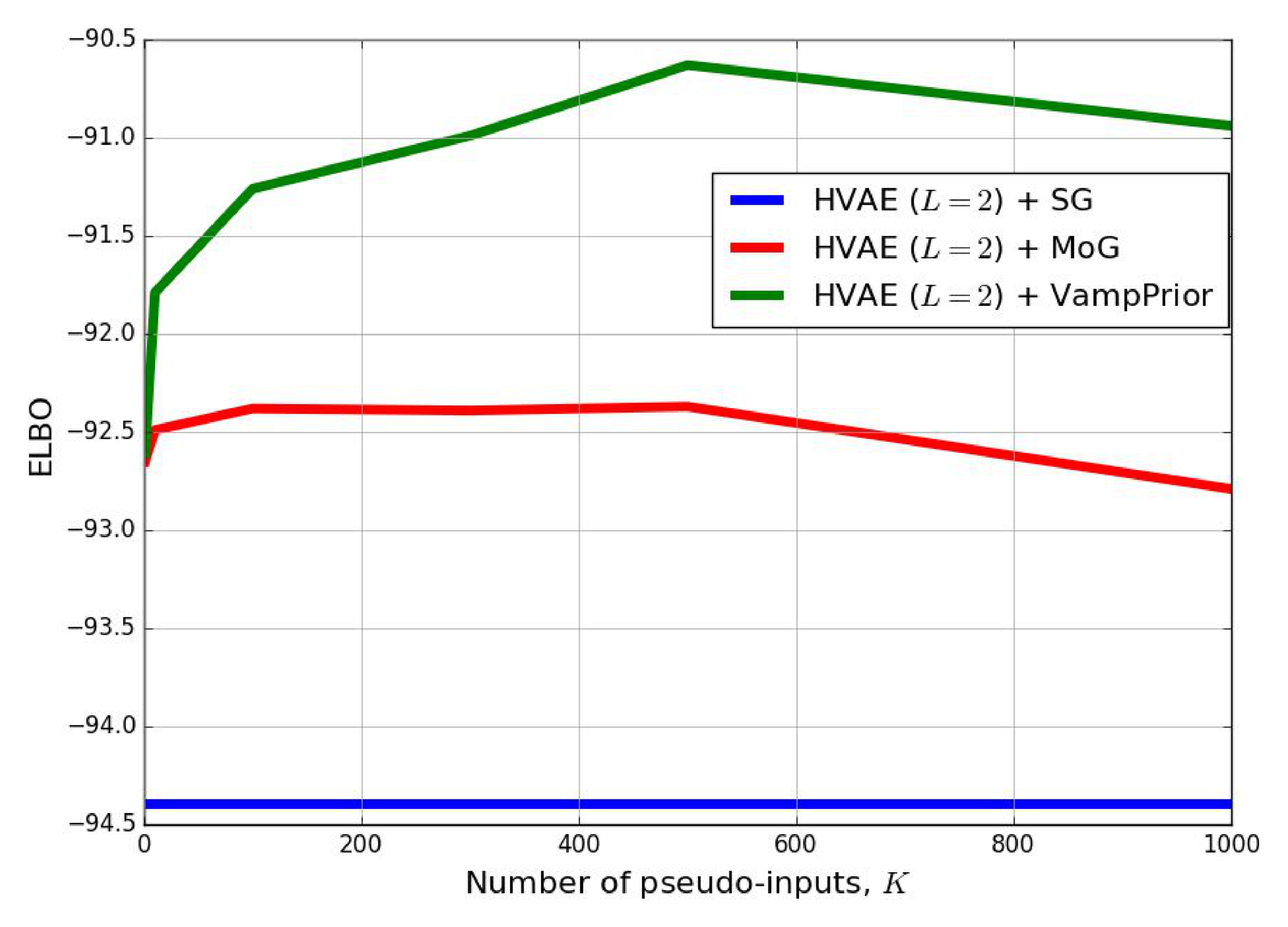
Additionally, we compared the VampPrior with the MoG prior and the SoG prior in Figure 2 for varying number of pseudo-inputs/components. Surprisingly, taking more pseudo-inputs does not help to improve the performance and, similarly, considering more mixture components also resulted in drop of the performance. However, again we can notice that the VampPrior is more flexible prior that outperforms the MoG.

An inspection of histograms of the log-likelihoods (see Supplementary Material) shows that the distributions of LL values are heavy-tailed and/or bimodal. A possible explanation for such characteristics of the histograms is the existence of many examples that are relatively simple to represent (first mode) and some really hard examples (heavy-tail). Comparing our approach to the VAE reveals that the VAE with the VampPrior is not only better on average but it produces less examples with high values of LL and more examples with lower LL.

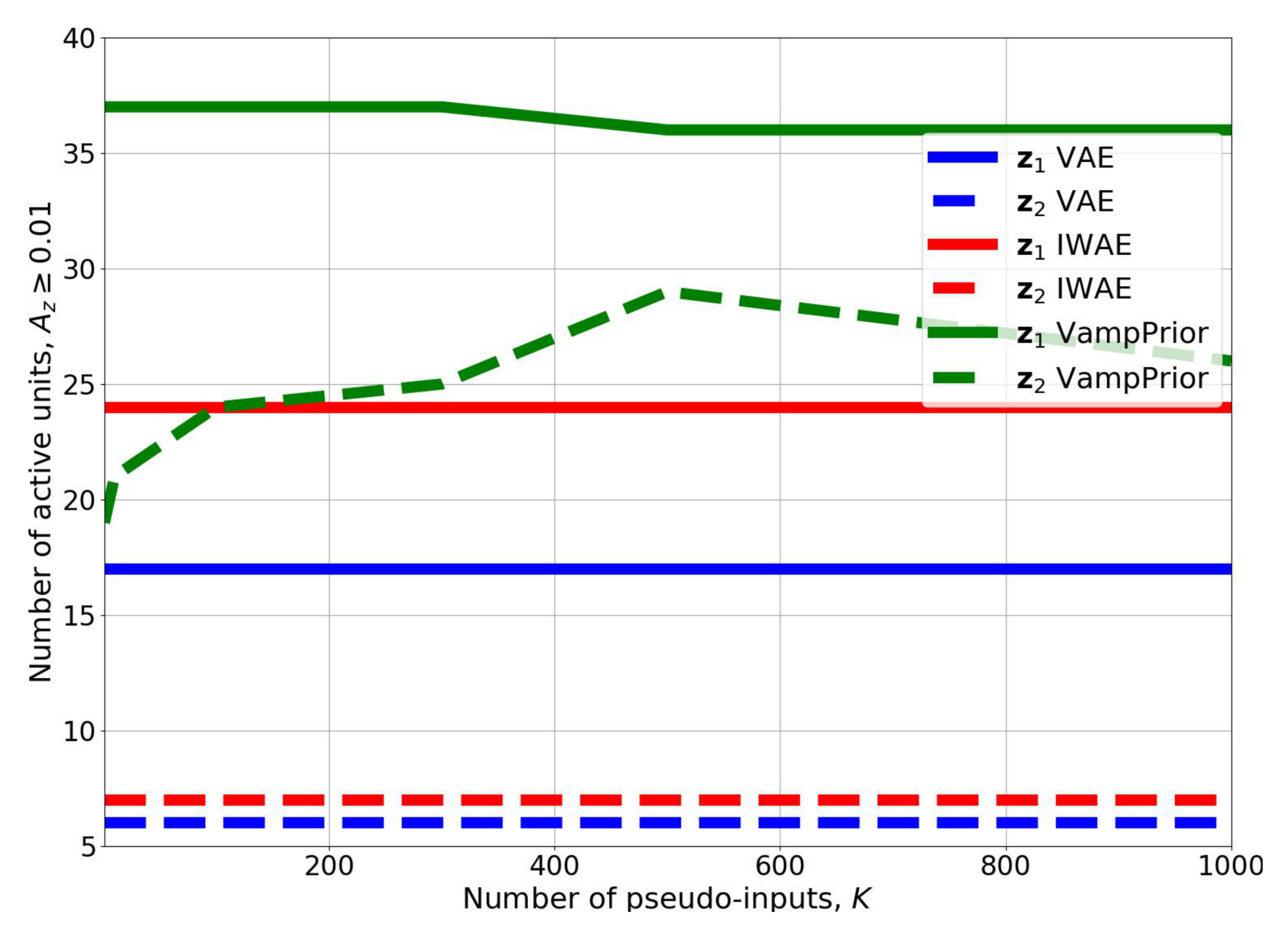
We hypothesized that the VampPrior provides a remedy for the inactive units issue. In order to verify this claim we utilized the statistics introduced in [15]. The results for the HVAE with the VampPrior in comparison to the two-level VAE and IWAE presented in [15] are given in Figure 3. The application of the VampPrior increases the number of active stochastic units four times for the second level and around 1.5 times more for the first level comparing to the VAE and the IWAE. Interestingly, the number of mixture components has a great impact on the number of active stochastic units in the second level. Nevertheless, even one mixture component allows to achieve almost three times more active stochastic units comparing to the vanilla VAE and the IWAE.

In general, an application of the VampPrior improves the performance of the VAE and in the case of two layers of stochastic units it yields the state-of-the-art results on all datasets for models that use MLPs. Moreover, our approach gets closer to the performance of models that utilize convolutional neural networks, such as, the one-layered VAE with the inverse autoregressive flow (IAF) [27] that achieves $-79.88$ on static MNIST and $-79.10$ on dynamic MNIST, the one-layered Variational Lossy Autoencoder (VLAE) [33] that obtains $-79.03$ on static MNIST and $-78.53$ on dynamic MNIST, and the hierarchical PixelVAE [35] that gets $-78.96$ on dynamic MNIST. On the other two datasets the VLAE performs way better than our approach with MLPs and achieves $-89.83$ on OMNIGLOT and $-77.36$ on Caltech 101 Silhouettes.

In order to compare our approach to the state-of-the-art convolutional-based VAEs we performed additional experiments using the HVAE ($L=2$) + VampPrior with convolutional layers in both the encoder and decoder. Next, we replaced the convolutional decoder with the PixelCNN [26] decoder ($\textsc{convHVAE}$ and $\textsc{PixelHVAE}$ in Table 2–Table 5). For the $\textsc{PixelHVAE}$ we were able to improve the performance to obtain $-79.78$ on static MNIST, $-78.45$ on dynamic MNIST, $-89.76$ on Omniglot, and $-86.22$ on Caltech 101 Silhouettes. The results confirmed that the VampPrior combined with a powerful encoder and a flexible decoder performs much better than the MLP-based approach and allows to achieve state-of-the-art performance on dynamic MNIST and OMNIGLOT[^2].

[^2]: In [33] the performance of the VLAE on static MNIST and Caltech 101 Silhouettes is provided for a different training procedure than the one used in this paper.

Qualitative results

The biggest disadvantage of the VAE is that it tends to produce blurry images [37]. We noticed this effect in images generated and reconstructed by VAE (see Supplementary Material). Moreover, the standard VAE produced some digits that are hard to interpret, blurry characters and very noisy silhouettes. The supremacy of HVAE + VampPrior is visible not only in LL values but in image generations and reconstructions as well because these are sharper.

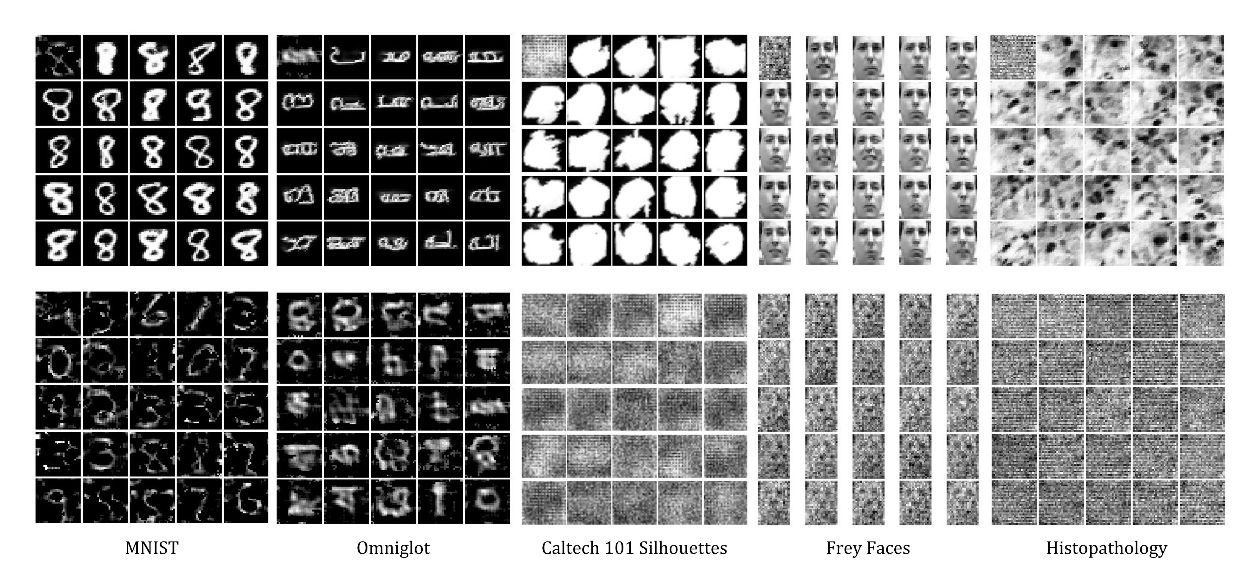
We also examine what the pseudo-inputs represent at the end of the training process (see Figure 4). Interestingly, trained pseudo-inputs are prototypical objects (digits, characters, silhouettes). Moreover, images generated for a chosen pseudo-input show that the model encodes a high variety of different features such as shapes, thickness and curvature for a single pseudo-input. This means that the model is not just memorizing the data-cases. It is worth noticing that for small-sample size and/or too flexible decoder the pseudo-inputs can be hard to train and they can represent noisy prototypes (e.g., see pseudo-inputs for Frey Faces in Figure 4).

6. Related work

Section Summary: Researchers have explored ways to improve variational autoencoders (VAEs) beyond their basic normal prior, such as using more complex priors like Dirichlet processes or autoregressive models, which enhance image generation but often require tricky training methods and can complicate assessing their true impact. Decoder architectures also play a key role in output quality, with suggestions like autoregressive networks or infinite mixtures boosting performance, though overly flexible decoders risk sidelining the encoder. Related studies include a concurrent memory-based VAE that shares some ideas with the VampPrior but lacks its explicit mixture and posterior coupling for better generation, while recent work shows the VampPrior excels in information-theoretic learning and can be refined with weights to avoid overfitting.

The VAE is a latent variable model that is usually trained with a very simple prior, i.e., the standard normal prior. In [38] a Dirichlet process prior using a stick-breaking process was proposed, while [39] proposed a nested Chinese Restaurant Process. These priors enrich the generative capabilities of the VAE, however, they require sophisticated learning methods and tricks to be trained successfully. A different approach is to use an autoregressive prior [33] that applies the IAF to random noise. This approach gives very promising results and allows to build rich representations. Nevertheless, the authors of [33] combine their prior with a convolutional encoder and an autoregressive decoder that makes it harder to assess the real contribution of the autoregressive prior to the generative model.

Clearly, the quality of generated images are dependent on the decoder architecture. One way of improving generative capabilities of the decoder is to use an infinite mixture of probabilistic component analyzers [40], which is equivalent to a rank-one covariance matrix. A more appealing approach would be to use deep autoregressive density estimators that utilize recurrent neural networks [26] or gated convolutional networks [41]. However, there is a threat that a too flexible decoder could discard hidden representations completely, turning the encoder to be useless [33].

Concurrently to our work, in [42] a variational VAE with a memory was proposed. This approach shares similarities with the VampPrior in terms of a learnable memory (pseudo-inputs in our case) and a multimodal prior. Nevertheless, there are two main differences. First, our prior is an explicit mixture while they sample components. Second, we showed that the optimal prior requires to be coupled with the variational posterior. In the experiments we showed that the VampPrior improves the generative capabilities of the VAE but in [42] it was noticed that the generative performance is comparable to the standard normal prior. We claim that the success of the VampPrior follows from the utilization of the variational posterior in the prior, a part that is missing in [42].

Very recently, the VampPrior was shown to be a perfect match for the information-theoretic approach to learn latent representation [19]. Additionally, the authors of [19] proposed to use a weighted version of the VampPrior:

$ p_{\lambda}(\mathbf{z}) = \sum_{k=1}^{K} w_{k} q_{\phi}(\mathbf{z}|\mathbf{u}_{k}), $

where $w_1, \ldots, w_K$ are trainable parameters such that $ \forall_k w_k \geq 0$ and $\sum_k w_k = 1$. This allows the VampPrior to learn which components (i.e, pseudo-inputs) are meaningful and may prevent from potential overfitting.

7. Conclusion

Section Summary: This paper proposes a new starting assumption, called the VampPrior, for improving variational autoencoders (VAEs), which are AI models that generate data like images by learning hidden patterns; it's built as a mixture of learned components limited by adjustable pseudo-inputs to keep it efficient. Using this in a two-layer generative model, the authors show it boosts performance on six datasets, resolves issues with underused hidden variables, and produces sharper generations and reconstructions than basic VAEs, matching or exceeding top results. They suggest exploring it for text and sound data or integrating it with techniques like normalizing flows, but plan to tackle those in future studies.

In this paper, we followed the line of thinking that the prior is a critical element to improve deep generative models, and in particular VAEs. We proposed a new prior that is expressed as a mixture of variational posteriors. In order to limit the capacity of the prior we introduced learnable pseudo-inputs as hyper-parameters of the prior, the number of which can be chosen freely. Further, we formulated a new two-level generative model based on this VampPrior. We showed empirically that applying our prior can indeed increase the performance of the proposed generative model and successfully overcome the problem of inactive stochastic latent variables, which is particularly challenging for generative models with multiple layers of stochastic latent variables. As a result, we achieved state-of-the-art or comparable results to SOTA models on six datasets. Additionally, generations and reconstructions obtained from the hierarchical VampPrior VAE are of better quality than the ones achieved by the standard VAE.

We believe that it is worthwhile to further pursue the line of the research presented in this paper. Here we applied our prior to image data but it would be interesting to see how it behaves on text or sound, where the sequential aspect plays a crucial role. We have already showed that combining the VampPrior VAE with convolutional nets and a powerful autoregressive density estimator is beneficial but more thorough study is needed. Last but not least, it would be interesting to utilize a normalizing flow [9], the hierarchical variational inference [43], ladder networks [34] or adversarial training [32] within the VampPrior VAE. However, we leave investigating these issues for future work.

Acknowledgements

The authors are grateful to Rianne van den Berg, Yingzhen Li, Tim Genewein, Tameem Adel, Ben Poole and Alex Alemi for insightful comments.

The research conducted by Jakub M. Tomczak was funded by the European Commission within the Marie Skłodowska-Curie Individual Fellowship (Grant No. 702666, ''Deep learning and Bayesian inference for medical imaging'').

8. SUPPLEMENTARY MATERIAL

Section Summary: This supplementary section provides detailed mathematical formulas for calculating gradients in a machine learning model's loss function, focusing on how changes to individual parameters affect the model for a single data point. It first derives the gradient for a standard normal prior distribution, then offers a version adapted for the VampPrior, a specialized prior used in variational methods. The final part breaks down the gradient computation step by step, splitting it into components related to data likelihood and prior terms to clarify the process.

8.1 The gradient of Equation 2a and 2b with the standard normal prior

The gradient of $\widetilde{ \mathcal{L} }(\phi, \theta, \lambda)$ in Equation (2a) and (2b) for the standard normal prior with respect to a single weight $\phi_{i}$ for a single data point $\mathbf{x}$ is the following:

$ \begin{align} \frac{\partial}{\partial \phi_i} \widetilde{ \mathcal{L} }(\mathbf{x}; \phi, \theta, \lambda) =& \frac{1}{L} \sum_{l=1}^{L} \Big[\frac{1}{ p_{\theta}(\mathbf{x}|\mathbf{z}{\phi}^{(l)})}\ \frac{\partial}{\partial \mathbf{z}{\phi} } p_{\theta}(\mathbf{x}|\mathbf{z}{\phi}^{(l)})\ \frac{\partial}{\partial \phi_i} \mathbf{z}{\phi}^{(l)} -\frac{1}{q_{\phi}(\mathbf{z}{\phi}^{(l)}|\mathbf{x})} \frac{\partial}{\partial \phi_i}q{\phi}(\mathbf{z}{\phi}^{(l)}|\mathbf{x}) + \tag{a} \ &+ \frac{1}{p{\lambda}(\mathbf{z}^{(l)}{\phi})\ q{\phi}(\mathbf{z}{\phi}^{(l)}|\mathbf{x})} \Big(q{\phi}(\mathbf{z}{\phi}^{(l)}|\mathbf{x}) \frac{\partial}{\partial \mathbf{z}{\phi} }p_{\lambda}(\mathbf{z}^{(l)}{\phi}) - p{\lambda}(\mathbf{z}^{(l)}{\phi}) \frac{\partial}{\partial \mathbf{z}{\phi} } q_{\phi}(\mathbf{z}{\phi}^{(l)}|\mathbf{x}) \Big) \frac{\partial}{\partial \phi_i} \mathbf{z}^{(l)}{\phi} \Big] . \tag{b} \end{align}\tag{7} $

8.2 The gradient of Equation 2a and 2b with the VampPrior

The gradient of $\widetilde{ \mathcal{L} }(\phi, \theta, \lambda)$ in Equation (2a) and (2b) for the VampPrior with respect to a single weight $\phi_{i}$ for a single data point $\mathbf{x}$ is the following:

$ \begin{align} \frac{\partial}{\partial \phi_i} \widetilde{ \mathcal{L} }(\mathbf{x}; \phi, \theta, \lambda) =& \frac{1}{L} \sum_{l=1}^{L} \Big[\frac{1}{ p_{\theta}(\mathbf{x}|\mathbf{z}{\phi}^{(l)})}\ \frac{\partial}{\partial \mathbf{z}{\phi} } p_{\theta}(\mathbf{x}|\mathbf{z}{\phi}^{(l)})\ \frac{\partial}{\partial \phi_i} \mathbf{z}{\phi}^{(l)} + \tag{a} \ &+ \frac{1}{K} \sum_{k=1}^{K} \Big{ \ \Big(\frac{q_{\phi}(\mathbf{z}{\phi}^{(l)} | \mathbf{x})\ \frac{\partial}{\partial \phi_i} q{\phi}(\mathbf{z}{\phi}^{(l)} | \mathbf{u}{k}) - q_{\phi}(\mathbf{z}{\phi}^{(l)} | \mathbf{u}{k})\ \frac{\partial}{\partial \phi_i} q_{\phi}(\mathbf{z}{\phi}^{(l)} | \mathbf{x})}{ \frac{1}{K} \sum{k=1}^{K} q_{\phi}(\mathbf{z}{\phi}^{(l)} | \mathbf{u}{k})\ q_{\phi}(\mathbf{z}{\phi}^{(l)} | \mathbf{x}) } \Big) + \tag{b} \ &+ \Big(\frac{ \big(q{\phi}(\mathbf{z}{\phi}^{(l)} | \mathbf{x})\ \frac{\partial}{\partial \mathbf{z}{\phi} } q_{\phi}(\mathbf{z}{\phi}^{(l)} | \mathbf{u}{k}) - q_{\phi}(\mathbf{z}{\phi}^{(l)} | \mathbf{u}{k})\ \frac{\partial}{\partial \mathbf{z}{\phi} } q{\phi}(\mathbf{z}{\phi}^{(l)} | \mathbf{x}) \big)\ \frac{\partial}{\partial \phi_i} \mathbf{z}{\phi}^{(l)} }{ \frac{1}{K} \sum_{k=1}^{K} q_{\phi}(\mathbf{z}{\phi}^{(l)} | \mathbf{u}{k})\ q_{\phi}(\mathbf{z}_{\phi}^{(l)} | \mathbf{x}) } \Big) \Big} \Big] . \tag{c} \end{align}\tag{8} $

8.3 Details on the gradient calculation in Equation 8b and 8c

Let us recall the objective function for single datapoint $\mathbf{x}_{*}$ using $L$ Monte Carlo sample points:

$ \widetilde{ \mathcal{L} }(\mathbf{x}{*}; \phi, \theta, \lambda) = \frac{1}{L} \sum{l=1}^{L} \Big[\ln p_{\theta}(\mathbf{x}{*}|\mathbf{z}{\phi}^{(l)}) \Big] + \frac{1}{L} \sum_{l=1}^{L} \Big[\ln \frac{1}{K} \sum_{k=1}^{K} q_{\phi}(\mathbf{z}{\phi}^{(l)} | \mathbf{u}{k}) - \ln q_{\phi}(\mathbf{z}{\phi}^{(l)}|\mathbf{x}{*}) \Big] .\tag{9} $

We are interested in calculating gradient with respect to a single parameter $\phi_i$. We can split the gradient into two parts:

$ \begin{align} \frac{\partial}{\partial \phi_i} \widetilde{ \mathcal{L} }(\mathbf{x}{*}; \phi, \theta, \lambda) =& \frac{\partial}{\partial \phi_i} \underbrace{ \frac{1}{L} \sum{l=1}^{L} \Big[\ln p_{\theta}(\mathbf{x}{*}|\mathbf{z}{\phi}^{(l)}) \Big] }{ (*) } \notag \ &+ \frac{\partial}{\partial \phi_i} \underbrace{ \frac{1}{L} \sum{l=1}^{L} \Big[\ln \frac{1}{K} \sum_{k=1}^{K} q_{\phi}(\mathbf{z}{\phi}^{(l)} | \mathbf{u}{k}) - \ln q_{\phi}(\mathbf{z}{\phi}^{(l)}|\mathbf{x}{*}) \Big] }_{ (**) } \end{align}\tag{10} $

Calculating the gradient separately for both $(*)$ and $(**)$ yields:

$ \begin{align} \frac{\partial}{\partial \phi_i} () &= \frac{\partial}{\partial \phi_i} \frac{1}{L} \sum_{l=1}^{L} \Big[\ln p_{\theta}(\mathbf{x}_{}|\mathbf{z}{\phi}^{(l)}) \Big] \notag \ &= \frac{1}{L} \sum{l=1}^{L} \frac{1}{ p_{\theta}(\mathbf{x}{*}|\mathbf{z}{\phi}^{(l)})}\ \frac{\partial}{\partial \mathbf{z}{\phi}} p{\theta}(\mathbf{x}{*}|\mathbf{z}{\phi}^{(l)})\ \frac{\partial}{\partial \phi_i} \mathbf{z}{\phi}^{(l)} \tag{a} \ & \notag\ \frac{\partial}{\partial \phi_i} (**)&= \frac{\partial}{\partial \phi_i} \frac{1}{L} \sum{l=1}^{L} \Big[\ln \frac{1}{K} \sum_{k=1}^{K} q_{\phi}(\mathbf{z}{\phi}^{(l)} | \mathbf{u}{k}) - \ln q_{\phi}(\mathbf{z}{\phi}^{(l)}|\mathbf{x}{}) \Big] \notag \ &[\text{Short-hand notation: } q_{\phi}(\mathbf{z}{\phi}^{(l)} | \mathbf{x}{}) \stackrel{\Delta}{=} q_{\phi}^{}, \quad q_{\phi}(\mathbf{z}{\phi}^{(l)} | \mathbf{u}{k}) \stackrel{\Delta}{=} q_{\phi}^{k}] \notag \ &= \frac{1}{L} \sum_{l=1}^{L} \Big[\frac{1}{ \frac{1}{K} \sum_{k=1}^{K} q_{\phi}^{k} }\ \Big(\frac{\partial}{\partial \phi_i} \frac{1}{K} \sum_{k=1}^{K} q_{\phi}^{k} + \frac{\partial}{\partial \mathbf{z}{\phi} } \big(\frac{1}{K} \sum{k=1}^{K} q_{\phi}^{k} \big)\ \frac{\partial}{\partial \phi_i} \mathbf{z}{\phi}^{(l)}\Big) + \notag\ &\quad - \frac{1}{ q{\phi}^{} }\ \Big(\frac{\partial}{\partial \phi_i} q_{\phi}^{} + \frac{\partial}{\partial \mathbf{z}{\phi} } q{\phi}^{}\ \frac{\partial}{\partial \phi_i} \mathbf{z}{\phi}^{(l)} \Big) \Big] \notag \ &= \frac{1}{L} \sum{l=1}^{L} \Big[\frac{1}{ \frac{1}{K} \sum_{k=1}^{K} q_{\phi}^{k}\ q_{\phi}^{} }\ \Big(\frac{1}{K} \sum_{k=1}^{K} q_{\phi}^{}\ \frac{\partial}{\partial \phi_i} q_{\phi}^{k} + \big(\frac{1}{K} \sum_{k=1}^{N} q_{\phi}^{}\ \frac{\partial}{\partial \mathbf{z}{\phi} } q{\phi}^{k} \big)\ \frac{\partial}{\partial \phi_i} \mathbf{z}{\phi}^{(l)}\Big) + \notag\ &\quad - \frac{1}{ \frac{1}{K} \sum{k=1}^{K} q_{\phi}^{k}\ q_{\phi}^{} }\ \Big(\frac{1}{K} \sum_{k=1}^{K} q_{\phi}^{k}\ \frac{\partial}{\partial \phi_i} q_{\phi}^{} + \frac{1}{K} \sum_{k=1}^{K} q_{\phi}^{k}\ \frac{\partial}{\partial \mathbf{z}{\phi} } q{\phi}^{}\ \frac{\partial}{\partial \phi_i} \mathbf{z}{\phi}^{(l)} \Big) \Big] \notag \ &= \frac{1}{L} \sum{l=1}^{L} \Big[\frac{1}{ \frac{1}{K} \sum_{k=1}^{K} q_{\phi}^{k}\ q_{\phi}^{} }\ \frac{1}{K} \sum_{k=1}^{K} \Big{ \ \Big(q_{\phi}^{}\ \frac{\partial}{\partial \phi_i} q_{\phi}^{k} - q_{\phi}^{k}\ \frac{\partial}{\partial \phi_i} q_{\phi}^{} \Big) + \notag\ &\quad + \Big(q_{\phi}^{}\ \frac{\partial}{\partial \mathbf{z}{\phi} } q{\phi}^{k} - q_{\phi}^{k}\ \frac{\partial}{\partial \mathbf{z}{\phi} } q{\phi}^{*} \Big)\ \frac{\partial}{\partial \phi_i} \mathbf{z}_{\phi}^{(l)} \Big} \Big] \tag{b} \end{align}\tag{11} $

For comparison, the gradient of $(**)$ for a prior $p_{\lambda}(\mathbf{z})$ that is independent of the variational posterior is the following:

$ \begin{align} & \frac{\partial}{\partial \phi_i} \Big[\frac{1}{L} \sum_{l=1}^{L} \ln p_{\lambda}(\mathbf{z}{\phi}^{(l)}) - \ln q{\phi}(\mathbf{z}{\phi}^{(l)}|\mathbf{x}{}) \Big] = \notag \ &[\text{Short-hand notation: } q_{\phi}(\mathbf{z}{\phi}^{(l)} | \mathbf{x}{}) \stackrel{\Delta}{=} q_{\phi}^{}, \qquad p_{\lambda}(\mathbf{z}{\phi}^{(l)}) \stackrel{\Delta}{=} p{\lambda}] \notag \ &= \frac{1}{L} \sum_{l=1}^{L} \Big[\frac{1}{ p_{\lambda} }\ \frac{\partial}{\partial \mathbf{z}{\phi} } p{\lambda}\ \frac{\partial}{\partial \phi_i} \mathbf{z}{\phi}^{(l)} - \frac{1}{ q{\phi}^{} }\ \Big(\frac{\partial}{\partial \phi_i} q_{\phi}^{} + \frac{\partial}{\partial \mathbf{z}{\phi} } q{\phi}^{}\ \frac{\partial}{\partial \phi_i} \mathbf{z}{\phi}^{(l)} \Big) \Big] \notag \ &= \frac{1}{L} \sum{l=1}^{L} \Big[- \frac{1}{ q_{\phi}^{} } \frac{\partial}{\partial \phi_i} q_{\phi}^{} + \frac{1}{ p_{\lambda}\ q_{\phi}^{} }\ \Big(q_{\phi}^{}\ \frac{\partial}{\partial \mathbf{z}{\phi}} p{\lambda} - p_{\lambda}\ \frac{\partial}{\partial \mathbf{z}{\phi}} q{\phi}^{*}\Big)\ \frac{\partial}{\partial \phi_i} \mathbf{z}_{\phi}^{(l)} \Big] \end{align}\tag{12} $

We notice that in Equation (11b) if $q_{\phi}^{} \approx q_{\phi}^{k}$ for some $k$, then the differences $(q_{\phi}^{}\ \frac{\partial}{\partial \phi_i} q_{\phi}^{k} - q_{\phi}^{k}\ \frac{\partial}{\partial \phi_i} q_{\phi}^{})$ and $(q_{\phi}^{}\ \frac{\partial}{\partial \mathbf{z}{\phi} } q{\phi}^{k} - q_{\phi}^{k}\ \frac{\partial}{\partial \mathbf{z}{\phi} } q{\phi}^{*})$ are close to $0$. Hence, the gradient points into an average of all dissimilar pseudo-inputs contrary to the gradient of the standard normal prior in Equation (12) that pulls always towards $\mathbf{0}$. As a result, the encoder is trained so that to have large variance because it is attracted by all dissimilar points and due to this fact it assigns separate regions in the latent space to each datapoint. This effect should help the decoder to decode a hidden representation to an image much easier.

8.4 Details on experiments

All experiments were run on NVIDIA TITAN X Pascal. The code for our models is available online at https://github.com/jmtomczak/vae_vampprior.

8.4.1 Datasets used in the experiments

We carried out experiments using six image datasets: static and dynamic MNIST^3, OMNIGLOT[^4] [23], Caltech 101 Silhouettes[^5] [24], Frey Faces^6, and Histopathology patches [11]. Frey Faces contains images of size $28 \times 20$ and all other datasets contain $28 \times 28$ images. We distinguish between static MNIST with fixed binarizartion of images [21] and dynamic MNIST with dynamic binarization of data during training as in [22].

[^4]: We used the pre-processed version of this dataset as in [15]: https://github.com/yburda/iwae/blob/master/datasets/OMNIGLOT/chardata.mat.

[^5]: We used the dataset with fixed split into training, validation and test sets: https://people.cs.umass.edu/~marlin/data/caltech101_silhouettes_28_split1.mat.

MNIST consists of hand-written digits split into 60, 000 training datapoints and 10, 000 test sample points. In order to perform model selection we put aside 10, 000 images from the training set. We distinguish between static MNIST with fixed binarizartion of images^7 [21] and dynamic MNIST with dynamic binarization of data during training as in [22].

OMNIGLOT is a dataset containing 1, 623 hand-written characters from 50 various alphabets. Each character is represented by about 20 images that makes the problem very challenging. The dataset is split into 24, 345 training datapoints and 8, 070 test images. We randomly pick 1, 345 training examples for validation. During training we applied dynamic binarization of data similarly to dynamic MNIST.

Caltech 101 Silhouettes contains images representing silhouettes of 101 object classes. Each image is a filled, black polygon of an object on a white background. There are 4, 100 training images, 2, 264 validation datapoints and 2, 307 test examples. The dataset is characterized by a small training sample size and many classes that makes the learning problem ambitious.

Frey Faces is a dataset of faces of a one person with different emotional expressions. The dataset consists of nearly 2, 000 gray-scaled images. We randomly split them into 1, 565 training images, $200$ validation images and $200$ test images. We repeated the experiment $3$ times.

Histopathology is a dataset of histopathology patches of ten different biopsies containing cancer or anemia. The dataset consists of gray-scaled images divided into 6, 800 training images, 2, 000 validation images and 2, 000 test images.

8.4.2 Additional results: Wall-clock times

Using our implementation, we have calculated wall-clock times for $K=500$ (measured on MNIST) and $K=1000$ (measured on OMNIGLOT). HVAE+VampPrior was about 1.4 times slower than the standard normal prior. ConvHVAE and PixelHVAE with the VampPrior resulted in the increased training times, respectively, by a factor of $\times 1.9$ / $\times 2.1$ and $\times 1.4$ / $\times 1.7$ ($K=500$ / $K=1000$) comparing to the standard prior. We believe that this time burden is acceptable regarding the improved generative performance resulting from the usage of the VampPrior.

8.4.3 Additional results: Generations, reconstructions and histograms of log-likelihood

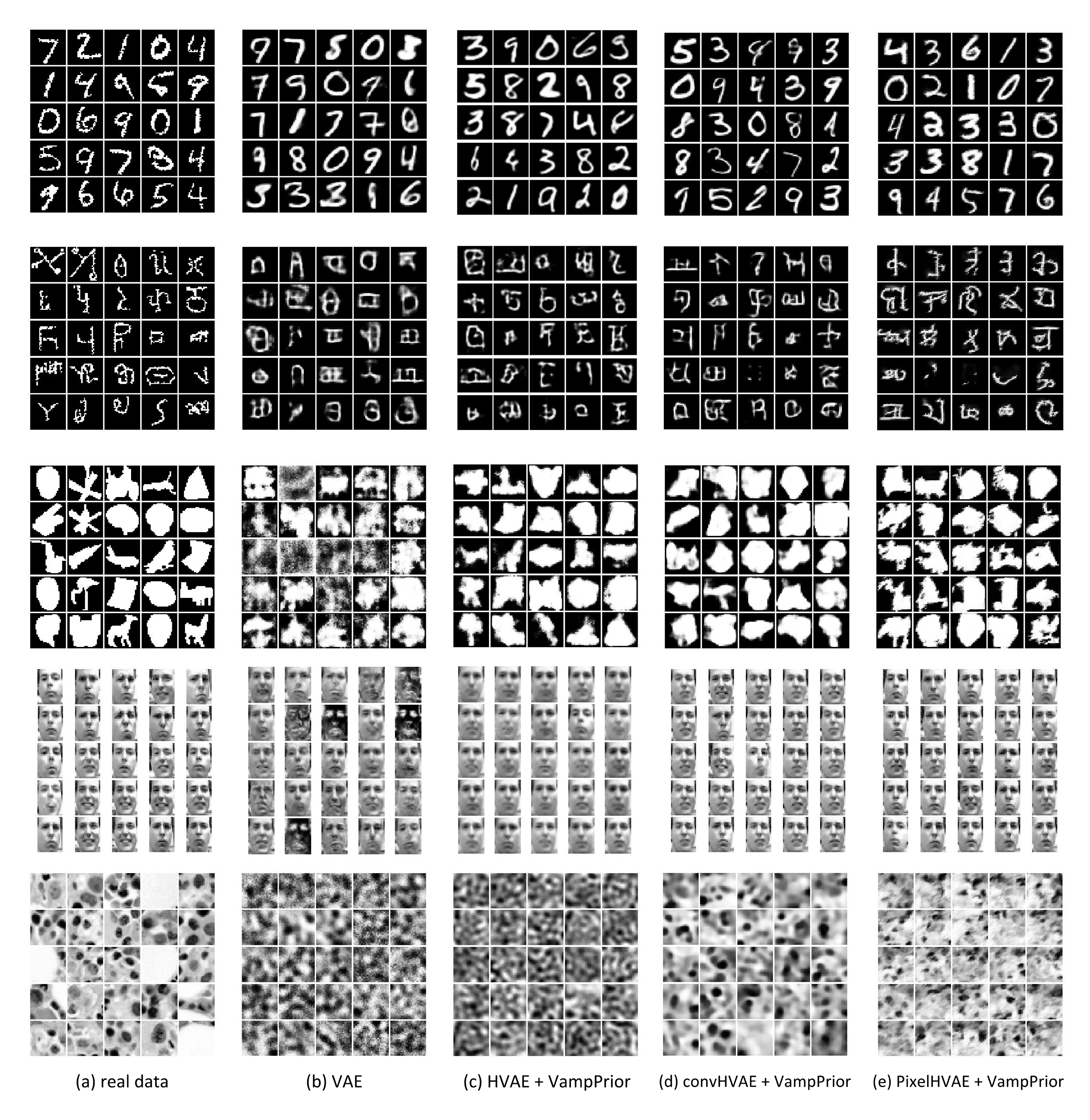
The generated images are presented in Figure 5. Images generated by HVAE ($L=2$) + VampPrior are more realistic and sharper than the ones given by the vanilla VAE. The quality of images generated by convHVAE and PixelHVAE contain much more details and better reflect variations in data.

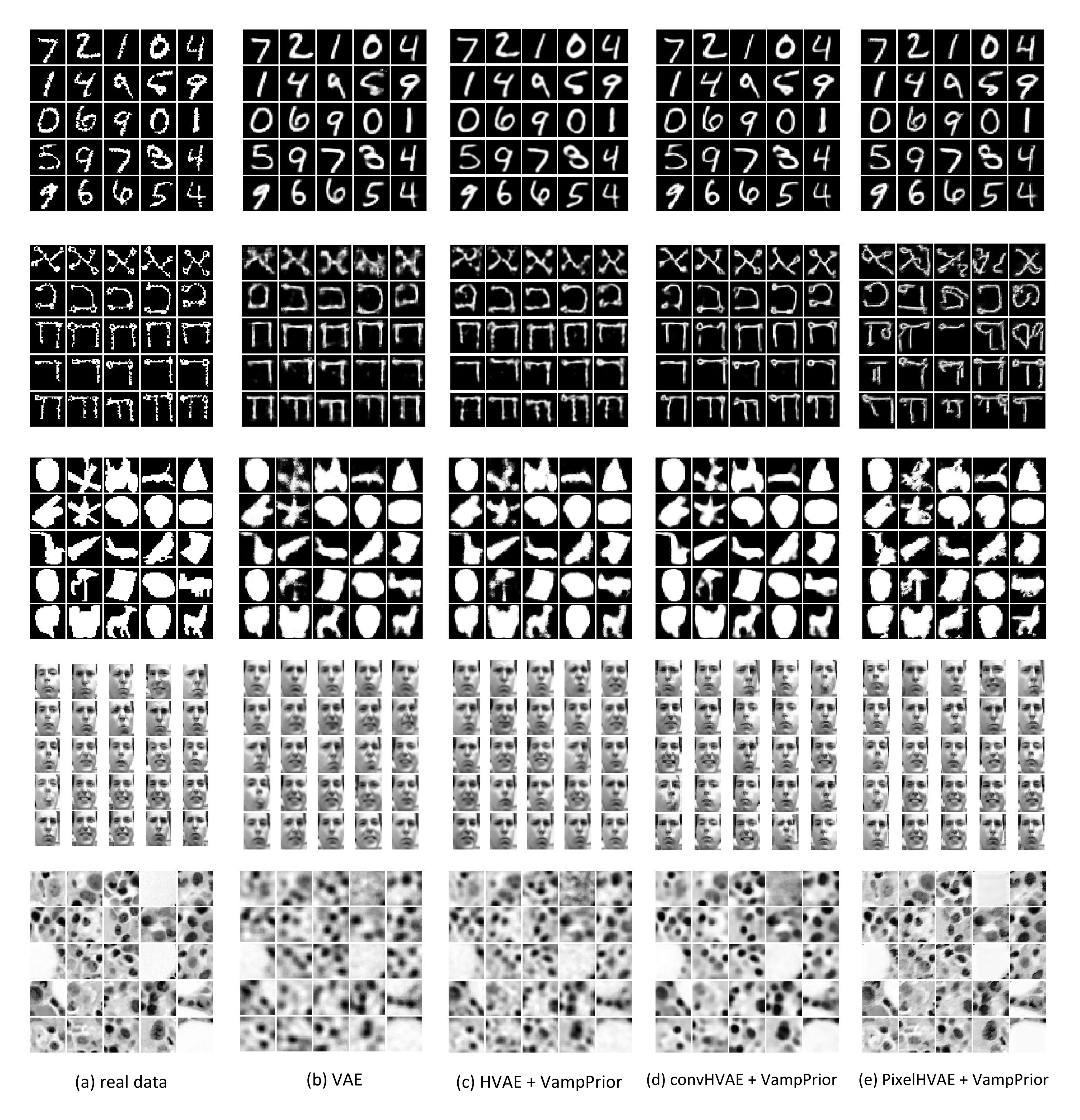
The reconstructions from test images are presented in Figure 6. At first glance the reconstructions of VAE and HVAE ($L=2$) + VampPrior look similarly, however, our approach provides more details and the reconstructions are sharper. This is especially visible in the case of OMNIGLOT (middle row in Figure 6) where VAE is incapable to reconstruct small circles while our approach does in most cases. The application of convolutional networks further improves the quality of reconstructions by providing many tiny details. Interestingly, for the PixelHVAE we can notice some "fantasizing" during reconstructing images (e.g., for OMNIGLOT). It means that the decoder was, to some extent, too flexible and disregarded some information included in the latent representation.

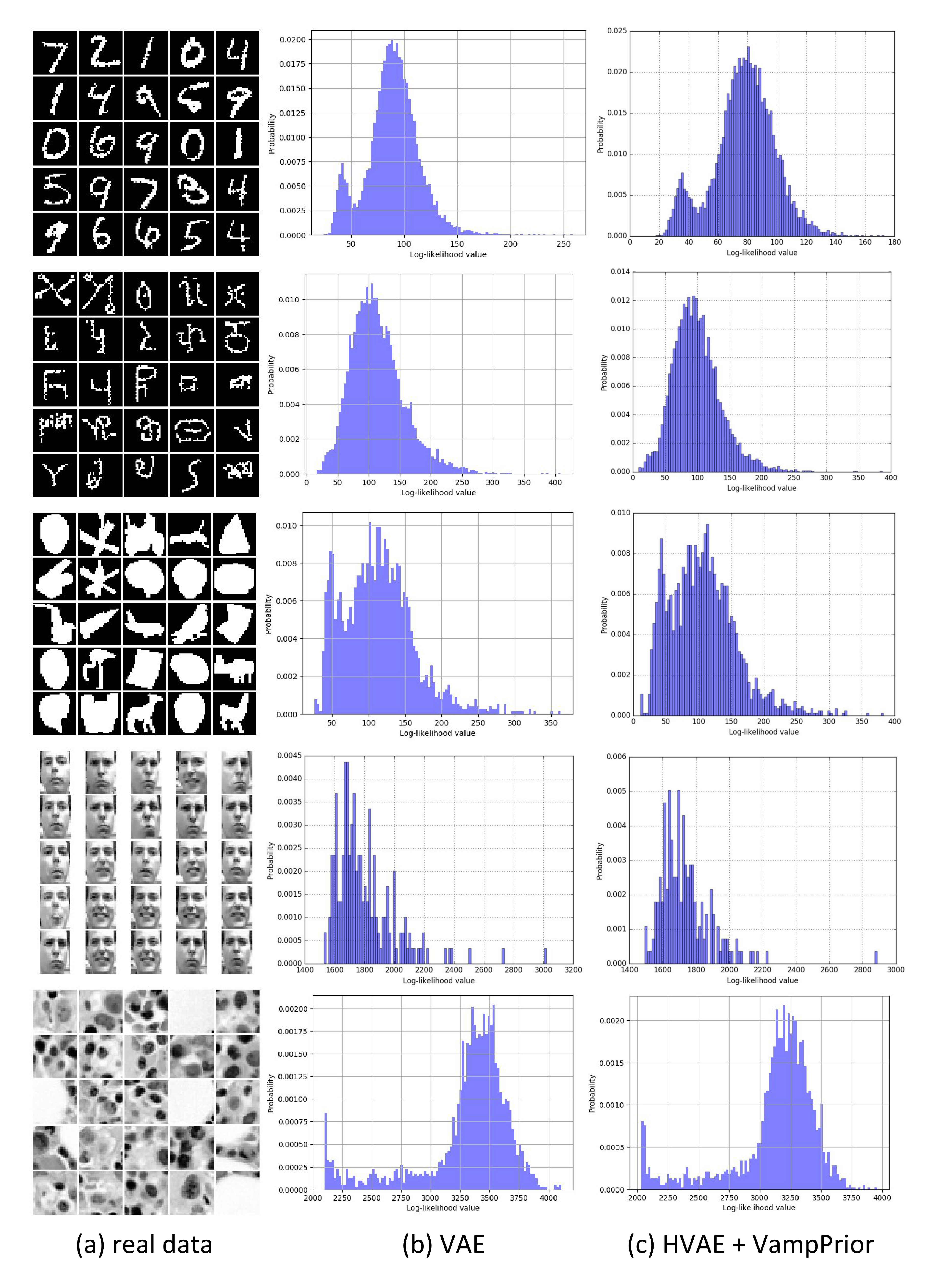
The histograms of the log-likelihood per test example are presented in Figure 7. We notice that all histograms characterize a heavy-tail indicating existence of examples that are hard to represent. However, taking a closer look at the histograms for HVAE ($L=2$) + VampPrior and its convolutional-based version reveals that there are less hard examples comparing to the standard VAE. This effect is especially apparent for the convHVAE.

References

Section Summary: This references section lists over 40 academic papers and preprints from 2000 to 2017, primarily focusing on advancements in machine learning techniques for generating data, such as neural networks, variational inference, and autoencoders. Key works include foundational papers on generative adversarial networks by Ian Goodfellow and variational autoencoders by Diederik Kingma, alongside contributions on improving inference methods and models for tasks like image and language generation. These citations draw from prestigious conferences like NIPS, ICML, and journals, providing the scholarly backbone for research in probabilistic and deep learning models.

[1] G. Dziugaite, D. Roy, and Z. Ghahramani. Training generative neural networks via maximum mean discrepancy optimization. UAI, pages 258–267, 2015.

[2] I. Goodfellow, J. Pouget-Abadie, M. Mirza, B. Xu, D. Warde-Farley, S. Ozair, A. Courville, and Y. Bengio. Generative adversarial nets. NIPS, pages 2672–2680, 2014.

[3] Y. Li, K. Swersky, and R. S. Zemel. Generative moment matching networks. ICML, pages 1718–1727, 2015.

[4] D. M. Blei, A. Kucukelbir, and J. D. McAuliffe. Variational inference: A review for statisticians. Journal of the American Statistical Association, 2017.

[5] D. P. Kingma and M. Welling. Auto-encoding variational bayes. arXiv:1312.6114, 2013.

[6] D. J. Rezende, S. Mohamed, and D. Wierstra. Stochastic Backpropagation and Approximate Inference in Deep Generative Models. ICML, pages 1278–1286, 2014.

[7] L. Dinh, D. Krueger, and Y. Bengio. NICE: Non-linear independent components estimation. arXiv:1410.8516, 2014.

[8] E. Nalisnick, L. Hertel, and P. Smyth. Approximate Inference for Deep Latent Gaussian Mixtures. NIPS Workshop: Bayesian Deep Learning, 2016.

[9] D. J. Rezende and S. Mohamed. Variational inference with normalizing flows. arXiv:1505.05770, 2015.

[10] T. Salimans, D. Kingma, and M. Welling. Markov chain monte carlo and variational inference: Bridging the gap. ICML, pages 1218–1226, 2015.

[11] J. M. Tomczak and M. Welling. Improving Variational Auto-Encoders using Householder Flow. NIPS Workshop: Bayesian Deep Learning, 2016.

[12] D. Tran, R. Ranganath, and D. M. Blei. The variational Gaussian process. arXiv:1511.06499, 2015.

[13] M. D. Hoffman and M. J. Johnson. ELBO surgery: yet another way to carve up the variational evidence lower bound. NIPS Workshop: Advances in Approximate Bayesian Inference, 2016.

[14] A. Makhzani, J. Shlens, N. Jaitly, I. Goodfellow, and B. Frey. Adversarial autoencoders. arXiv:1511.05644, 2015.

[15] Y. Burda, R. Grosse, and R. Salakhutdinov. Importance weighted autoencoders. arXiv:1509.00519, 2015.

[16] N. Dilokthanakul, P. A. Mediano, M. Garnelo, M. C. Lee, H. Salimbeni, K. Arulkumaran, and M. Shanahan. Deep unsupervised clustering with gaussian mixture variational autoencoders. arXiv:1611.02648, 2016.

[17] A. Alemi, I. Fischer, J. Dillon, and K. Murphy. Deep variational information bottleneck. ICLR, 2017.

[18] N. Tishby, F. C. Pereira, and W. Bialek. The information bottleneck method. arXiv preprint physics/0004057, 2000.

[19] A. A. Alemi, B. Poole, I. Fischer, J. V. Dillon, R. A. Saurous, and K. Murphy. An information-theoretic analysis of deep latent-variable models. arXiv preprint arXiv:1711.00464, 2017.

[20] L. Maaløe, M. Fraccaro, and O. Winther. Semi-supervised generation with cluster-aware generative models. arXiv:1704.00637, 2017.

[21] H. Larochelle and I. Murray. The Neural Autoregressive Distribution Estimator. AISTATS, 2011.

[22] R. Salakhutdinov and I. Murray. On the quantitative analysis of deep belief networks. ICML, pages 872–879, 2008.

[23] B. M. Lake, R. Salakhutdinov, and J. B. Tenenbaum. Human-level concept learning through probabilistic program induction. Science, 350(6266):1332–1338, 2015.

[24] B. Marlin, K. Swersky, B. Chen, and N. Freitas. Inductive principles for Restricted Boltzmann Machine learning. AISTATS, pages 509–516, 2010.

[25] Y. N. Dauphin, A. Fan, M. Auli, and D. Grangier. Language Modeling with Gated Convolutional Networks. arXiv:1612.08083, 2016.

[26] A. van den Oord, N. Kalchbrenner, and K. Kavukcuoglu. Pixel Recurrent Neural Networks. ICML, pages 1747–1756, 2016.

[27] D. P. Kingma, T. Salimans, R. Jozefowicz, X. Chen, I. Sutskever, and M. Welling. Improved variational inference with inverse autoregressive flow. NIPS, pages 4743–4751, 2016.

[28] D. Kingma and J. Ba. Adam: A method for stochastic optimization. arXiv:1412.6980, 2014.

[29] A. W. Yu, Q. Lin, R. Salakhutdinov, and J. Carbonell. Normalized gradient with adaptive stepsize method for deep neural network training. arXiv:1707.04822, 2017.

[30] S. R. Bowman, L. Vilnis, O. Vinyals, A. M. Dai, R. Jozefowicz, and S. Bengio. Generating sentences from a continuous space. arXiv:1511.06349, 2016.

[31] X. Glorot and Y. Bengio. Understanding the difficulty of training deep feedforward neural networks. AISTATS, 9:249–256, 2010.

[32] L. Mescheder, S. Nowozin, and A. Geiger. Adversarial Variational Bayes: Unifying Variational Autoencoders and Generative Adversarial Networks. In ICML, pages 2391–2400, 2017.

[33] X. Chen, D. P. Kingma, T. Salimans, Y. Duan, P. Dhariwal, J. Schulman, I. Sutskever, and P. Abbeel. Variational Lossy Autoencoder. arXiv:1611.02731, 2016.

[34] C. K. Sønderby, T. Raiko, L. Maaløe, S. K. Sønderby, and O. Winther. Ladder variational autoencoders. NIPS, pages 3738–3746, 2016.

[35] I. Gulrajani, K. Kumar, F. Ahmed, A. A. Taiga, F. Visin, D. Vazquez, and A. Courville. PixelVAE: A latent variable model for natural images. arXiv:1611.05013, 2016.

[36] Y. Li and R. E. Turner. Rényi Divergence Variational Inference. NIPS, pages 1073–1081, 2016.

[37] A. B. L. Larsen, S. K. Sønderby, H. Larochelle, and O. Winther. Autoencoding beyond pixels using a learned similarity metric. ICML, 2016.

[38] E. Nalisnick and P. Smyth. Stick-Breaking Variational Autoencoders. arXiv:1605.06197, 2016.

[39] P. Goyal, Z. Hu, X. Liang, C. Wang, and E. Xing. Nonparametric Variational Auto-encoders for Hierarchical Representation Learning. arXiv:1703.07027, 2017.

[40] S. Suh and S. Choi. Gaussian Copula Variational Autoencoders for Mixed Data. arXiv:1604.04960, 2016.

[41] A. van den Oord, N. Kalchbrenner, L. Espeholt, O. Vinyals, A. Graves, and K. Kavukcuoglu. Conditional image generation with PixelCNN decoders. NIPS, pages 4790–4798, 2016.

[42] J. Bornschein, A. Mnih, D. Zoran, and D. J. Rezende. Variational Memory Addressing in Generative Models. arXiv:1709.07116, 2017.

[43] R. Ranganath, D. Tran, and D. Blei. Hierarchical variational models. In ICML, pages 324–333, 2016.